The YOLO (You Only Look Once) family of models continues to grow and right after YOLOv6 was released, YOLOv7 was delivered quickly after. The most recent introduction is MT-YOLOv6, or as the authors say, "YOLOv6 for brevity."
Be sure to open the YOLOv6 Custom Training Colab Notebook alongside this guide
The YOLOv6 repository was published June 2022 by Meituan, and it claims new state-of-the-art performance on the COCO dataset benchmark. We'll leave it to the community to determine if this name is the best representation for the architecture. (We saw how engaged the machine learning community gets about naming at the time of comparing YOLOv5 vs YOLOv4.)
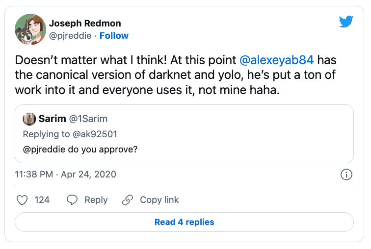
And who could forget that Joseph Redmon, author of the original YOLO models (the first three iterations), said he's not especially concerned with names when YOLOv4 was released:
In any case, it's clear MT-YOLOv6 (hereafter YOLOv6 for brevity) is popular. In a couple short weeks, the repo has attracted over 2,000+ stars and 300+ forks. Let's dive in to how to train YOLOv6 on a custom dataset. The custom dataset we'll be using for this post is Chess Piece Detection. (You can find your own custom dataset from the 90,000+ the Roboflow community have shared on Roboflow Universe.)
In this post, we'll cover all you need to train YOLOv6:
- Install YOLOv6 dependencies
- Creating a custom dataset for YOLOv6
- Convert annotations to the YOLOv6 annotation format
- Load custom object detection data for YOLOv6
- Configure YOLOv6 model training options
- Train a custom YOLOv6 model
- Evaluate YOLOv6 performance
- Run YOLOv6 inference on test images
- Convert YOLOv6 to ONNX
- Apply active learning to improve YOLOv6 performance
We'll wrap this guide with a bit about What's New in YOLOv6 as well.
Installing YOLOv6 Dependencies
If you haven't yet, be sure to open up the YOLOv6 custom training notebook to follow along with this guided tutorial.
To get started, we need to clone the YOLOv6 repository and install its dependencies. This will setup our development environment with the required machine learning libraries to train YOLOv6. Perhaps of note, YOLOv6 is based in PyTorch, and the requirements.txt calls for torch>=1.8.0.
!git clone https://github.com/meituan/YOLOv6
%cd YOLOv6
!pip install -r requirements.txt
(If you're curious, in Colab, we can also always check which GPU has been allocated to us by running !nvidia-smi. Odds are you'll be allocated a Tesla P100.)
Creating a Custom Dataset to Train YOLOv6
A model – even the newest state of the art object detection model – is only as good as the dataset. Thus, it's critically important to prepare high quality images and annotations for your training. Good images (and video) are ones that are representative of the view your model will see in production. The closer to reality your training data is, the better the model will perform.
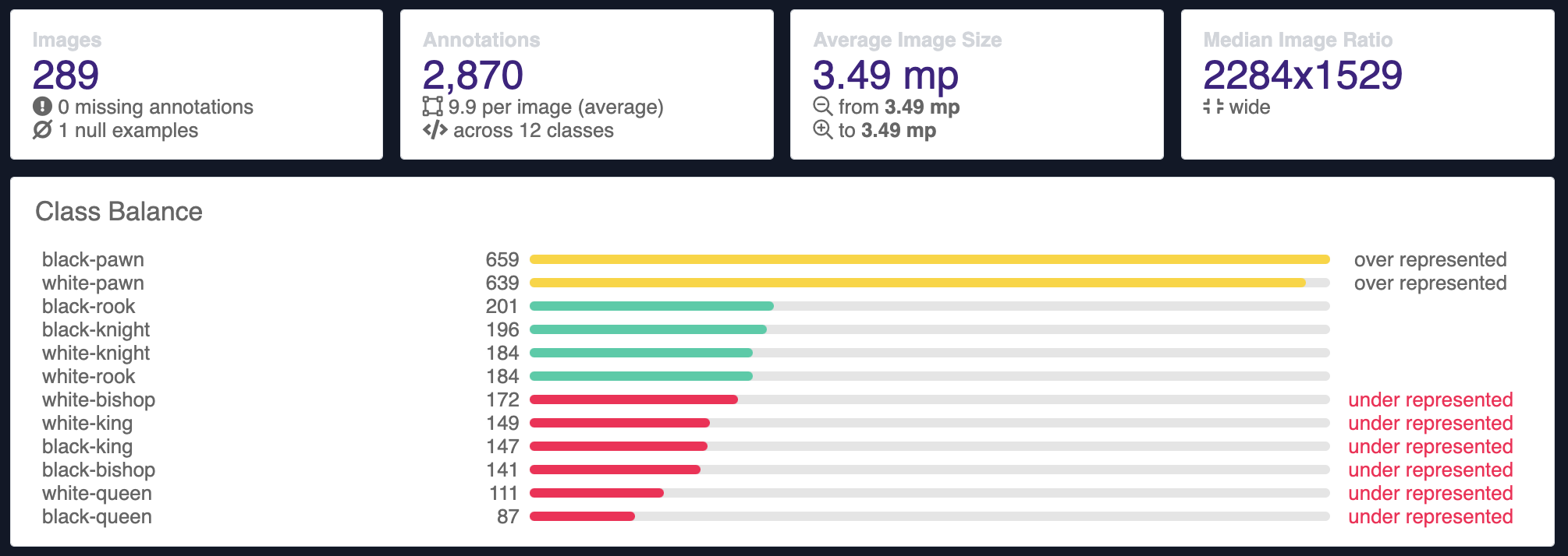
In our custom chess piece detection tutorial, our images already come with 2,870 annotations across 289 images (thanks, open source datasets!). You can jump to the next header section if you plan to proceed with this chess dataset, or use any of the thousands of object detection datasets that are open source computer vision datasets from Roboflow Universe.
Labeling and Annotation for YOLOv6
If your images are not yet labeled, they can be annotated using Roboflow Annotate, a free and powerful annotation tool. Other free tools include CVAT and labelimg.
Label and Annotate Data with Roboflow for free
Use Roboflow to manage datasets, label data, and convert to 26+ formats for using different models. Roboflow is free up to 10,000 images, cloud-based, and easy for teams.
Roboflow Annotate makes it easy to have a model assist with labeling, share and assign labeling tasks to others, and annotate with fewer clicks. To get started, login at https://roboflow.com, create a new Workspace, and select the free Public plan.
Labeling images with Roboflow Annotate
Good annotations are consistent, tight bounding boxes with 200+ examples per class (and this figure varies widely based on the variance in the classes being detected). For more tips on ensuring your dataset is high quality (like what to do about partial objects), be sure to check out Seven Tips for Labeling Images for Computer Vision:
Convert Annotations to the YOLOv6 Annotation Format
Whether you labeled images from scratch or you already have images and annotations, correctly converting those images into the format that work with YOLOv6 is essential to smooth training.
Computer vision annotation formats come in many varieties. The most common are COCO JSON, Pascal VOC XML, and the YOLO TXT format. Roboflow supports annotation conversion among 30+ formats (and counting!).
About the YOLOv6 Annotation Format
YOLOv6 introduces a slightly new dataset configuration format. The authors use a specific directory hierarchy, custom .yaml format, and the YOLO TXT format for individual image annotations.
This is the directory structure YOLOv6 expects looks like the following:
# image directory
path/to/data/images/train/im0.jpg
path/to/data/images/val/im1.jpg
path/to/data/images/test/im2.jpg

# label directory
path/to/data/labels/train/im0.txt
path/to/data/labels/val/im1.txt
path/to/data/labels/test/im2.txt
The directory format for YOLOv6.
The directory structure calls for a parent directory of images with the train, val, and test splits each containing their respective batch of images. The labels follow a similar pattern.
The corresponding YOLOv6 YAML file is structured like this:
train: ./images/train
val: ./images/valid
test: ./images/test

nc: 12
names: ['black-bishop', 'black-king', 'black-knight', 'black-pawn', 'black-queen', 'black-rook', 'white-bishop', 'white-king', 'white-knight', 'white-pawn', 'white-queen', 'white-rook']
The YAML format for YOLOv6.
Here, we're defining the location of our train, validation, and testing directories. We're stating the number of classes (nc) , and we're listing the names of those classes.
And the individual image annotations are the YOLO TXT format, like this:
# class_id center_x center_y bbox_width bbox_height
3 0.6033653846153846 0.2439903846153846 0.051682692307692304 0.12980769230769232
The YOLO TXT format that YOLOv6 uses.
The YOLO TXT format is not especially intuitive without an example. Every image has a corresponding text file with its annotation location. The above text file corresponds to the below image. The text file indicates the class ID (in this case, black-knight happens to be class 3), and the relative location of the bounding box's center (x,y) and size (width, height). The numeric values are relative to the images' size and distance from an upper left (0,0) origin (i.e. the bottom right hand pixel location is (1,1) and everything in between will be a value between (0-1).
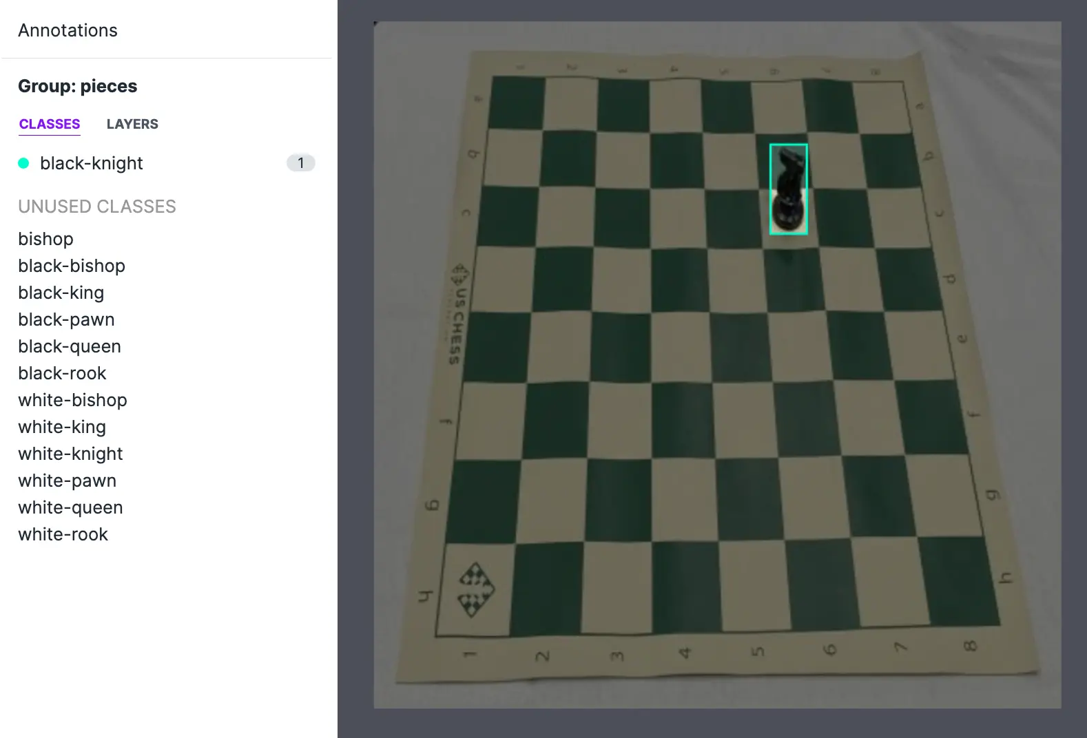
Ensuring your annotations are well maintained is one of the best ways to improve model performance and reduce errors.
Let's walkthrough how to convert annotations to YOLOv6, including generating the correct directory structure and YAML file so we can load them into our YOLOv6 custom training notebook.
Roboflow enables easy conversion to this format so you can ensure your annotations are formatted correctly and your model trains easily.
Step-by-Step: Converting to YOLOv6 Annotations
If you'd like to follow this tutorial with the chess detection dataset instead of your own, simply use this link to use the YOLOv6 formatted chess data.
To format your own data into the YOLOv6 annotation format, proceed here's how. If you haven't yet, create a free Roboflow account on https://roboflow.com.
Ensuring your annotations do not have errors is critical to preventing silent model failure. 100,000+ developers trust Roboflow to get it right.
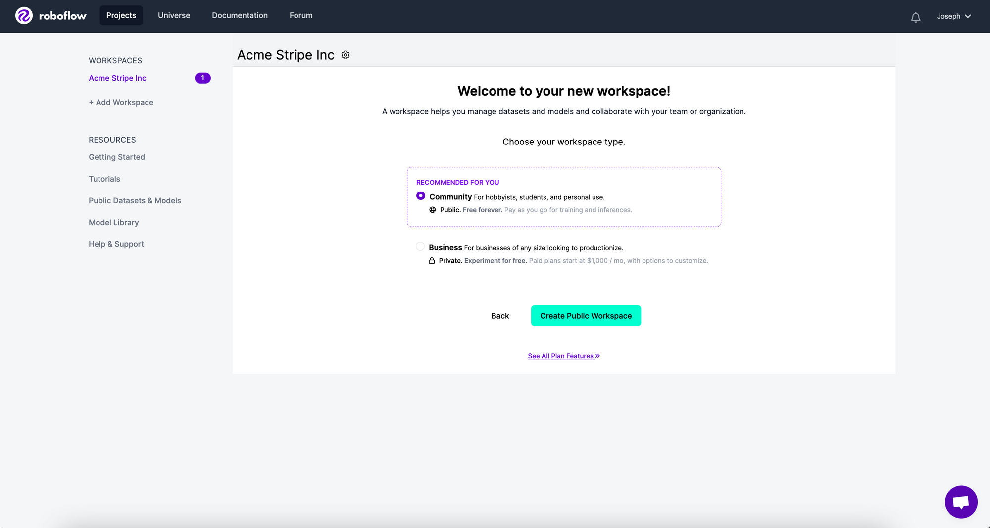
Then, we'll create a new Workspace. Invite those you may want to collaborate with, and select Community. This Public plan enables higher usage limits and easy integration for custom training models like YOLOv6.
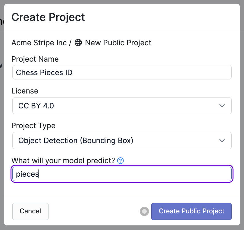
Create a New Project, and select Upload Your Own Data. Name your Project and be sure it's Object Detection (as YOLOv6 is an object detection model).
Now you can drop in annotations of nearly any type (COCO JSON, VOC XML, Scale, etc) no matter where you annotated them. Roboflow will automatically match the images and annotations as well as perform rule-based quality assurance (i.e. annotations accidentally beyond image edges).
Roboflow will automatically read and match our images and annotations.
Click upload and follow the 70/20/10 train test split. Our YOLOv6 notebook will expect to see train, valid, and test directories.
Now that we have our images and annotations added, we can Generate a Dataset Version. (And if any images still require annotations, feel free to add those at this point, too) When Generating a Version, you may elect to add preprocessing and augmentations. These are entirely up to you – our YOLOv6 tutorial does not require them (though you may be able to get a boost in performance).
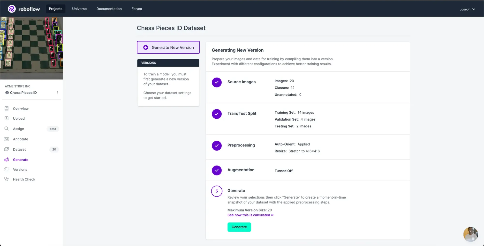
Once the dataset version is generated, we have a hosted dataset we can load directly into our notebook for easy training.
Simply click Export and select the meituan/YOLOv6 dataset format.
Select "Show Download Code" for the meituan/YOLOv6 format.
Hang on to this code snippet! We'll need it in our notebook.
Load Custom Object Detection Data for YOLOv6
Now that we've got our data in the right directories format, loading it into our training pipeline is a simple copy/paste. In the YOLOv6 Custom Training Notebook, there's a section for "Download Correctly Formatted Custom Data." In that code cell below, the notebook encourages pasting in a code snippet.
The code snippet to paste here is the one we generated above. (Or simply grab the chess dataset code snippet from here.)
# REPLACE with your custom code snippet generated above

!pip install roboflow

from roboflow import Roboflow
rf = Roboflow(api_key="YOUR_API_KEY")
project = rf.workspace("YOUR_WORKSPACE").project("YOUR_PROJECT")
dataset = project.version(1).download("mt-yolov6")
Paste your code snippet here.
Your data is automatically formatted into the correct directory structure, the YAML file is correct, and your annotations are in the correct YOLO TXT format. Proceed to train!
Configure YOLOv6 Custom Training Options
YOLOv6 supports a number of custom training options for things like the size of model (YOLOv6-n, YOLOv6-tiny, YOLOv6s – m/l/x are coming soon), single or multi GPU support, fine tuning a training job vs starting from scratch, and a high number of custom training parameters to affect your training.
In our example notebook, we'll make use of single GPU support.
# training with single GPU support
python tools/train.py --batch 256 --conf configs/yolov6s_finetune.py --data data/data.yaml --device 0

# training with mutli GPU support
python -m torch.distributed.launch --nproc_per_node 4 tools/train.py --batch 256 --conf configs/yolov6s_finetune.py --data data/data.yaml --device 0,1,2,3
YOLOv6 supports training both on single GPU and multi GPU.
Note the structure of the basic training command: we call a specific script (tools/train.py), set a batch size argument (--batch 256), set a specific configuration file (--conf configs/yolov6s.py), pass our data.yaml file, and set what type of CUDA device we're using (--device 0).
The configuration file for training YOLOv6 comes with support for finetuning (e.g. calling configs/yolov6s_finetune.py vs starting from scratch (yolov6s.py). Finetuning will train faster though may not be as effective on unique datasets. It may make most sense if you're resuming training from a substantially similar domain, like adding more data to a previously completed training job.
Moreover, YOLOv6 supports a high number of arguments by default. Here's what all the options available to us are, their default value, and what they mean:
--data-path, default='./data/coco.yaml', type=str, help='path of dataset')--conf-file,default='./configs/yolov6s.py', type=str, help='experiments description file')--img-size, type=int, default=640, help='train, val image size (pixels)')--batch-size, default=32, type=int, help='total batch size for all GPUs')--epochs, default=400, type=int, help='number of total epochs to run')--workers, default=8, type=int, help='number of data loading workers (default: 8)')--device, default='0', type=str, help='cuda device, i.e. 0 or 0,1,2,3 or cpu')--eval-interval, type=int, default=20, help='evaluate at every interval epochs')--eval-final-only, action='store_true', help='only evaluate at the final epoch')--heavy-eval-range, default=50,help='evaluating every epoch for last such epochs (can be jointly used with --eval-interval)')--check-images, action='store_true', help='check images when initializing datasets')--check-labels, action='store_true', help='check label files when initializing datasets')--output-dir, default='./runs/train', type=str, help='path to save outputs')--name, default='exp', type=str, help='experiment name, saved to output_dir/name')--dist_url, type=str, default="default url: tcp://127.0.0.1:8888")--gpu_count, type=int, default=0)--local_rank, type=int, default=-1, help='DDP parameter')--resume, type=str, default=None, help='resume the corresponding ckpt')
YOLOv6 is still under active development, so expect the training to continue to change and introduce new arguments.
Train a Custom YOLOv6 Model
Alas, we're ready to kickoff our training command in the notebook. In our example, we opted to slightly modify the baseline training command. We'll pass this:
!python tools/train.py --batch 32 --conf configs/yolov6s.py --epochs 100 --img-size 416 --data {dataset.location}/data.yaml --device 0 Our training command ✨
Note that we're adjusting the default epochs from 400 to 100. This is to expedite results. We're also adjusting the image size from the default 600x600 to 416x416. This is partially to increase training speed and also to keep in-line with prior YOLO family model norms (for easier head-to-head comparisons of performance).
Lastly, we set an intelligent environment variable {dataset.location} to enable our exported dataset to find the correct YOLOv6 format.
Note that adjusting parameters like lower batch size and smaller image sizes can also help with low memory. With Colab, the above parameters yielded results.
When our chess piece detection model finished 400 epochs in 1.157 hours, it posted a mAP@0.50 of 0.985 (comparable to YOLOv5 on the same dataset for those wondering – indicating this task is maxing out performance).
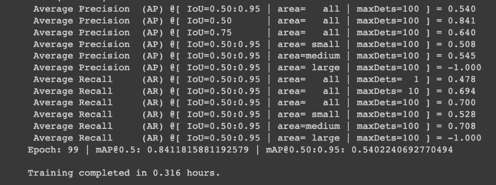
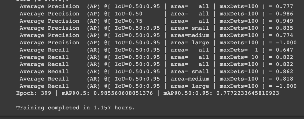
On the left, the results on our chess dataset after 100 epochs (0.84 mAP@0.50 in 0.316 hours). On the right, the results on our chess dataset after 400 epochs (0.985 mAP@0.50 in 1.157 hours).
Evaluate YOLOv6 Model Performance
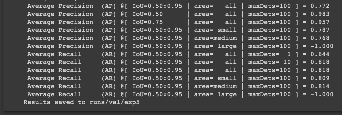
YOLOv6 comes with a tools directory, one of which is for evaluation of model training. Evaluating the model's performance includes assessing the model's mean average precision (mAP), precision, and recall. For the uninitiated, a higher mAP score indicates our model is drawing the correct boxes in the right places.
Similar to the training argument, we do have parameters we can adjust for how we evaluate the model (like specifying confidence thresholds or modifying where the results are saved).
--data, type=str, default='./data/coco.yaml', help='dataset.yaml path')-weights, type=str, default='./weights/yolov6s.pt', help='model.pt path(s)')--batch-size, type=int, default=32, help='batch size')--img-size, type=int, default=640, help='inference size (pixels)')--conf-thres, type=float, default=0.001, help='confidence threshold')--iou-thres, type=float, default=0.65, help='NMS IoU threshold')--task, default='val', help='val, or speed')--device, default='0', help='cuda device, i.e. 0 or 0,1,2,3 or cpu')--half, default=False, action='store_true', help='whether to use fp16 infer')--save_dir, type=str, default='runs/val/', help='evaluation save dir')-name, type=str, default='exp', help='save evaluation results to save_dir/name')
The evaluation command we'll run is:
!python tools/eval.py --data {dataset.location}/data.yaml --img-size 416 --weights runs/train/exp/weights/best_ckpt.pt --device 0
Notably, we're grabbing our dataset's .yaml file from the right location (this ensures the model knows what images to run evaluation on), setting image size to 416 (as we did in training), and specifying which weights to use (the path here is the default path for where model training saved them.
The evaluation JSON output saves in the runs directory for the validation set and reports the results.
Inference with YOLOv6 on Test Images
There's nothing quite like seeing your model infer on your own data! It shows all the hard work has paid off (hopefully).
Similar to YOLOv6 evaluation, there's an inference script that comes with the repository's tools. This inference script allows us to pass a batch of images in a given directory on which the model will run its predictions.
In addition, this inference utility also comes with a number of arguments we can pass for things like displaying the labels on the predicted images (which is on by default), modifying the confidence level and NMS thresholds, and setting max detections.
--weights, type=str, default='weights/yolov6s.pt', help='model path(s) for inference.')--source, type=str, default='data/images', help='the source path, e.g. image-file/dir.')--yaml, type=str, default='data/coco.yaml', help='data yaml file.')--img-size, type=int, default=640, help='the image-size(h,w) in inference size.')--conf-thres, type=float, default=0.25, help='confidence threshold for inference.')--iou-thres, type=float, default=0.45, help='NMS IoU threshold for inference.')--max-det, type=int, default=1000, help='maximal inferences per image.')--device, default='0', help='device to run our model i.e. 0 or 0,1,2,3 or cpu.')--save-txt, action='store_true', help='save results to *.txt.')--save-img, action='store_false', help='save visuallized inference results.')--classes, nargs='+', type=int, help='filter by classes, e.g. --classes 0, or --classes 0 2 3.')--agnostic-nms, action='store_true', help='class-agnostic NMS.')--project, default='runs/inference', help='save inference results to project/name.')-name, default='exp', help='save inference results to project/name.')--hide-labels, default=False, action='store_true', help='hide labels.')--hide-conf, default=False, action='store_true', help='hide confidences.')--half, action='store_true', help='whether to use FP16 half-precision inference.')
We'll run this command:
!python tools/infer.py --yaml {dataset.location}/data.yaml --img-size 416 --weights runs/train/exp/weights/best_ckpt.pt --source {dataset.location}/images/test/ --device 0
Here, we're again ensuring we have our dataset labels correctly loaded by referencing our .yaml, set image size to 416 to remain consistent with training, specify where our weights are, and point the inference script at our test set. If this errors for you, a first thing to check is ensuring you created a correct test set in when splitting your data. (You can always Generate a New Version in Roboflow with a new Train, Valid, Test split.)
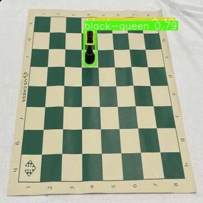
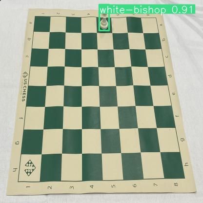
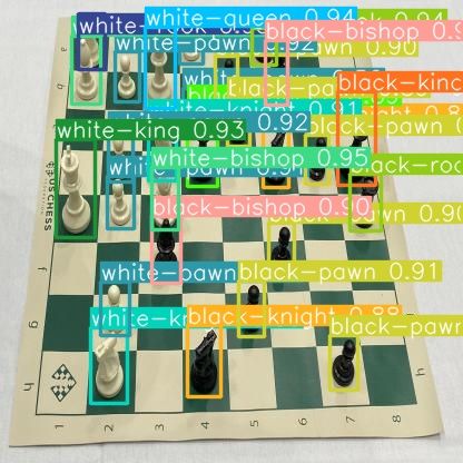
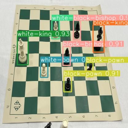
A sampling of inferences after training for 100 epochs. The model appears to have taken to the task, albeit it could be more robust on a few predictions. More training time and a slightly higher confidence threshold would do the trick.
Convert YOLOv6 to ONNX
One additional utility YOLOv6 comes with is the ability to be converted to ONNX, a common model serialization format for easier portability across devices.
Converting to ONNX is a simple command, where we've correctly references our model's weights file:
python deploy/ONNX/export_onnx.py --weights runs/train/exp/weights/best_ckpt.pt --device 0
Active Learning with YOLOv6
Training (and even deploying) is truly only the beginning, however. Once a model has been trained, we should make use of active learning to smartly and quickly improve our model. This will lessen the data labeling and prep requirements while also improving our model's performance.
The recommended way to setup active learning is to create simple rules that automatically store and re-upload individual frames/images from key moments. For example, if the model sees an underrepresented class or makes a prediction below a given confidence threshold, we should use that image to add back to our source dataset.
As an example, here's how to connect a Python project to make programmatic uploads back to your Roboflow project.
# setup access to your workspace
rf = Roboflow(api_key="YOUR_API_KEY")                               # used above to load data
inference_project =  rf.workspace().project("YOUR_PROJECT_NAME")    # used above to load data
model = inference_project.version(1).model

upload_project = rf.workspace().project("YOUR_PROJECT_NAME")

print("inference reference point: ", inference_project)
print("upload destination: ", upload_project)
Now that we've made our way through the notebook, let's address a few things new in YOLOv6.
YOLOv6: What's New?
Similar to the authors of YOLOv5, the authors of YOLOv6 have yet to publish a paper detailing specific changes to the architecture. This suggests YOLOv6 will also be continuously improving as an ongoing repository rather than being a snapshot of a model in time.
COCO Benchmark Performance
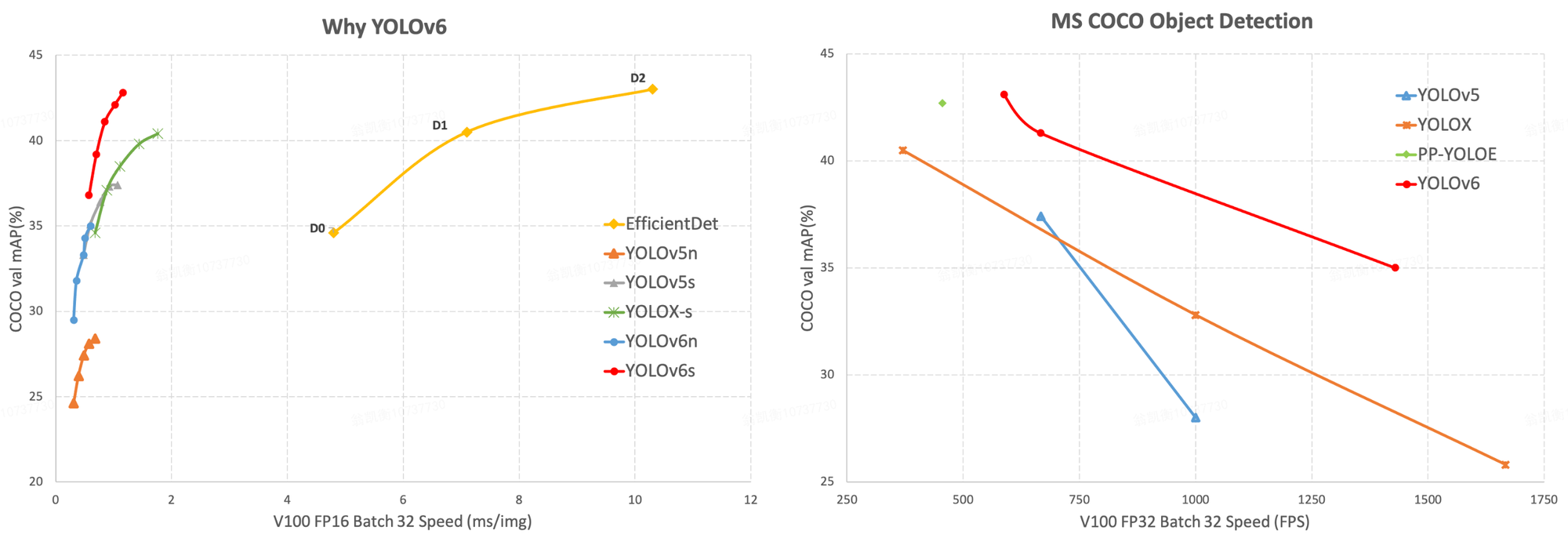
YOLOv6 claims to set a new state-of-the-art performance on the COCO dataset benchmark. As the authors detail, YOLOv6-s achieves 43.1 mAP on COCO val2017 dataset (with 520 FPS on T4 using TensorRT FP16 for bs32 inference).
(For point of comparison, YOLOv5-s achieves 37.4 mAP @ 0.95% on the same COCO benchmark.)
The YOLOv6 repository authors published the below evaluation graphic, demonstrating YOLOv6 outperforming YOLOv5 and YOLOX at similar sizes.
YOLOv6 Architecture and Innovation
The YOLOv6 authors note that a couple of key innovations are introduced in their model, including efficient decoupled head with SIoU loss and "hardware friendly design" for Backbone and Neck. Architectural diagrams depicting the networks layers are yet to be published. Stay tuned for a deeper dive.
YOLOv6 Sizes - YOLOv6n, YOLOv6t, and YOLOv6s
At the time of release, YOLOv6 is available in three sizes: YOLOv6n, YOLOv6t, and YOLOv6s (nano, tiny, and small, respectively). How big is YOLOv6? Absent quantization, YOLOv6-nano is a mere 9.8 MB and 4.3M parameters, YOLOv6-tiny is 33 MB and 15M parameters, and YOLOv6-small is 38.1 MB and 17.2M parameters.
The authors note that the larger YOLOv6 m/l/x models are coming soon.

(For point of size comparison, YOLOv5-small is 15 MB and 7.2 million parameters.)
Please share this post if you found it helpful, and let us know your feedback. Happy training!
Cite this Post
Use the following entry to cite this post in your research:
Joseph Nelson. (Jul 1, 2022). How to Train a YOLOv6 Model on a Custom Dataset. Roboflow Blog: https://blog.roboflow.com/how-to-train-yolov6-on-a-custom-dataset/

