
Capturing the intensity of elite sports requires a delicate equilibrium between processing speed and spatial accuracy. In the high-stakes world of sports broadcasting and media production, the ability to follow the action in real-time is the ultimate goal for quality engagement. A single missed tackle or an obscured jersey number on a game-winning drive can lead to lost narrative moments and the broadcaster's greatest fear: a failed highlight delivery.
Traditionally, logging player movements and identifying highlights relied on manual video review, a workflow plagued by human exhaustion and delayed turnaround times. Today, computer vision is revolutionizing the arena. By utilizing AI, media crews can deploy automated systems that monitor every inch of the turf with digital precision.
In this article, we will examine how to build a tracking pipeline that transforms broadcast footage into searchable metadata using Roboflow’s ecosystem.
How to do American Football Player Tracking
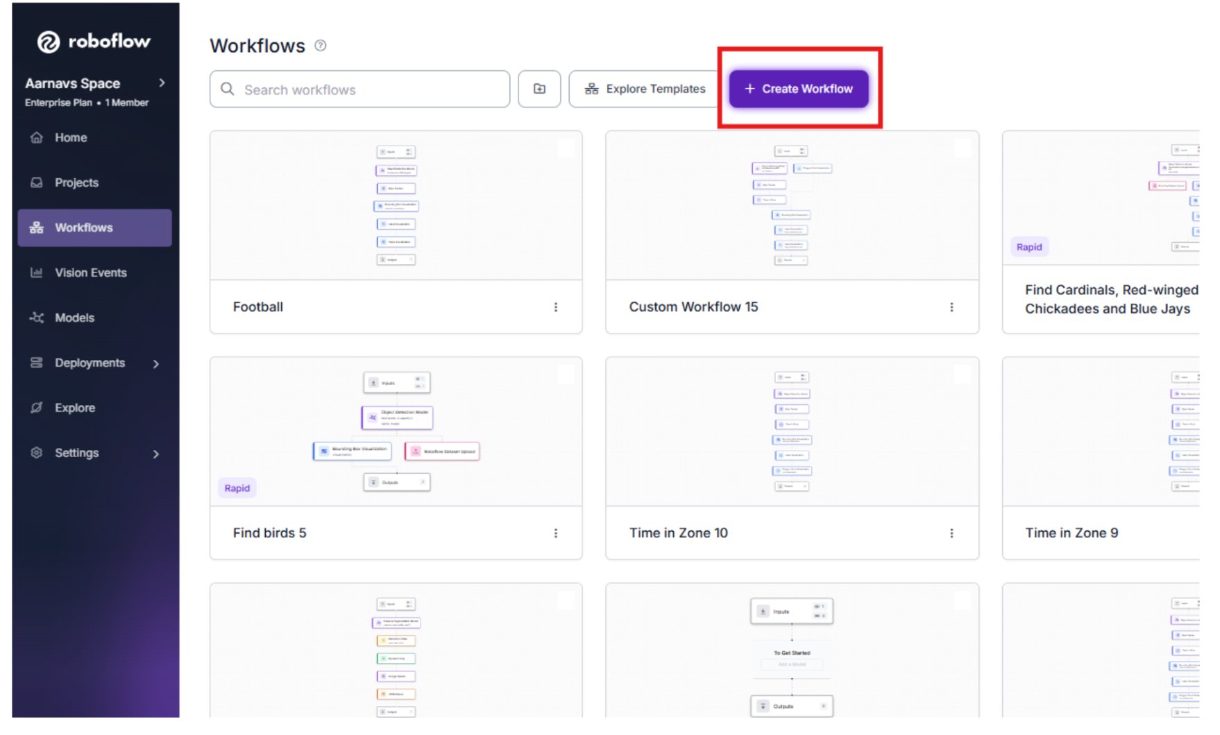
Step 1: Log in to Roboflow
Organize your development environment by signing into Roboflow. If you are starting fresh, you can register for a free account to begin organizing your sports-centric vision projects.
Step 2: Import the Dataset
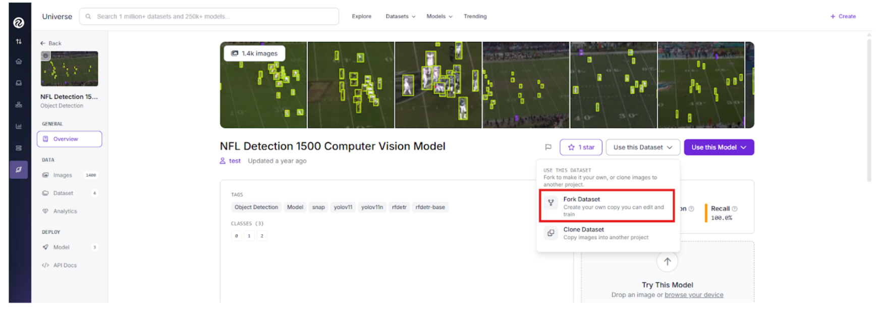
Effective machine learning begins with domain-specific data. We will use an American Football dataset from Roboflow Universe, which is curated for recognizing jersey patterns and various stadium lighting conditions.
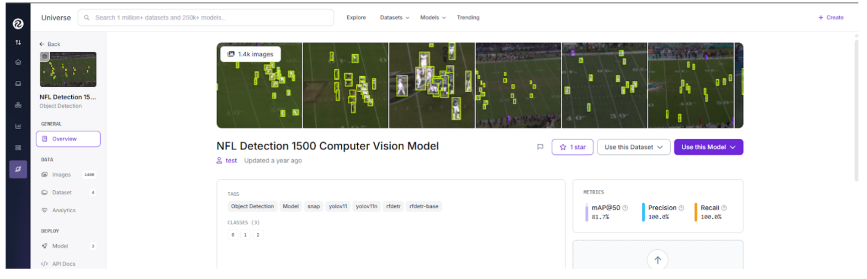
Search for a football tracking project on Universe and click "Fork Project" to pull the source imagery into your personal workspace for custom training.
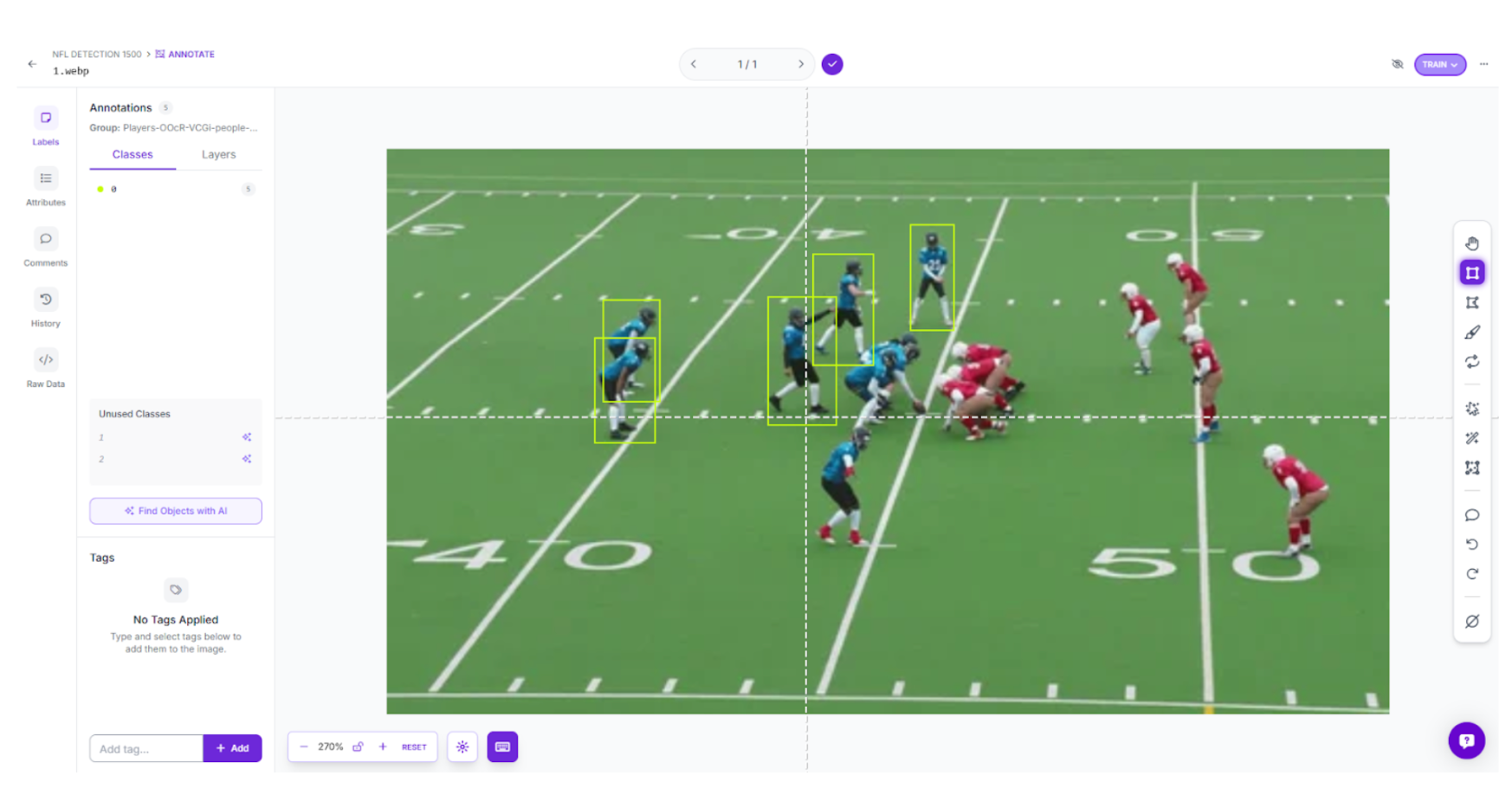
Step 3: Labeling and Annotation
When working with your specific game footage, use Roboflow’s annotation tools to establish your targets. Generate precise boxes around players, labeling them by team or role to provide the model with a clear taxonomy.
Step 4: Train the RF-DETR Object Detection Model
We are employing Roboflow's RF-DETR architecture for our detection core. As a leading transformer model capable of high-speed inference, it provides the low-latency precision necessary for live sports.
- Initiate Training: Navigate to the "Train" tab in your project dashboard.
- Select Your Framework: Choose the RF-DETR Object Detection (Small) version.
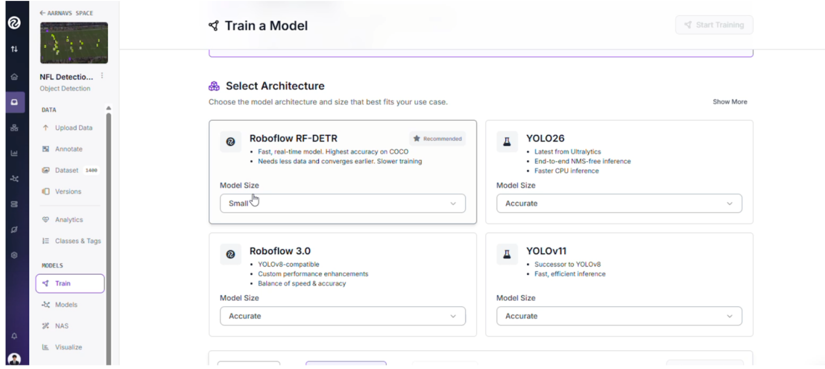
The Strategy Behind RF-DETR Small: While larger variants offer more parameters, the "Small" version is the tactical choice for this live-production pipeline:
- Instantaneous Inference: Broadcast feeds require millisecond processing; this model ensures inference occurs fast enough to keep up with the live action.
- Edge Portability: It is compact enough to be deployed on local hardware like an NVIDIA Jetson, keeping the compute local to the stadium.
Step 5: Configure your Train/Test Split
When preparing our football data, we utilized a standard distribution to ensure the model generalizes well across different games:
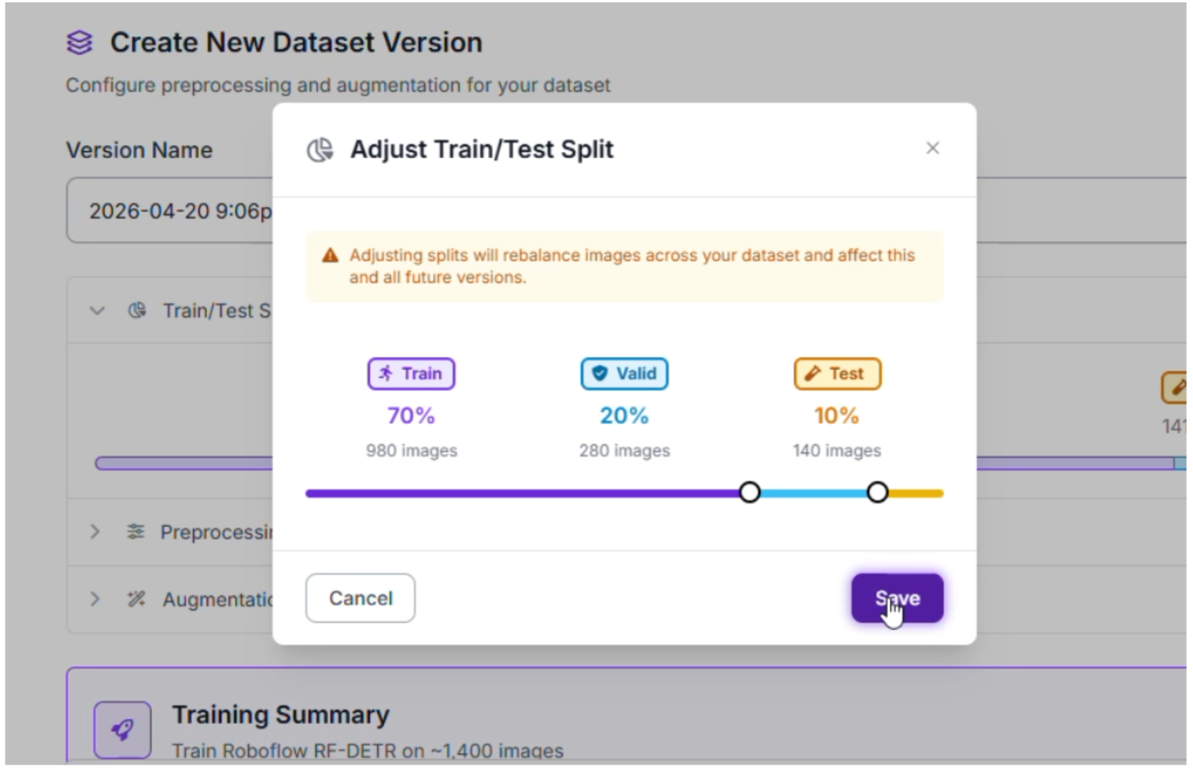
- Training Set (70%): Provides the model with thousands of examples of jersey colors, helmets, and turf textures.
- Validation Set (20%): Used to fine-tune hyperparameters and prevent the model from simply memorizing specific stadium layouts.
- Testing Set (10%): Acts as the final exam, evaluating how the detector handles a match it has never encountered before.
Step 6: Apply Preprocessing and Augmentations
To ensure our tracker remains resilient against motion blur and varied camera angles, we applied the following augmentations:
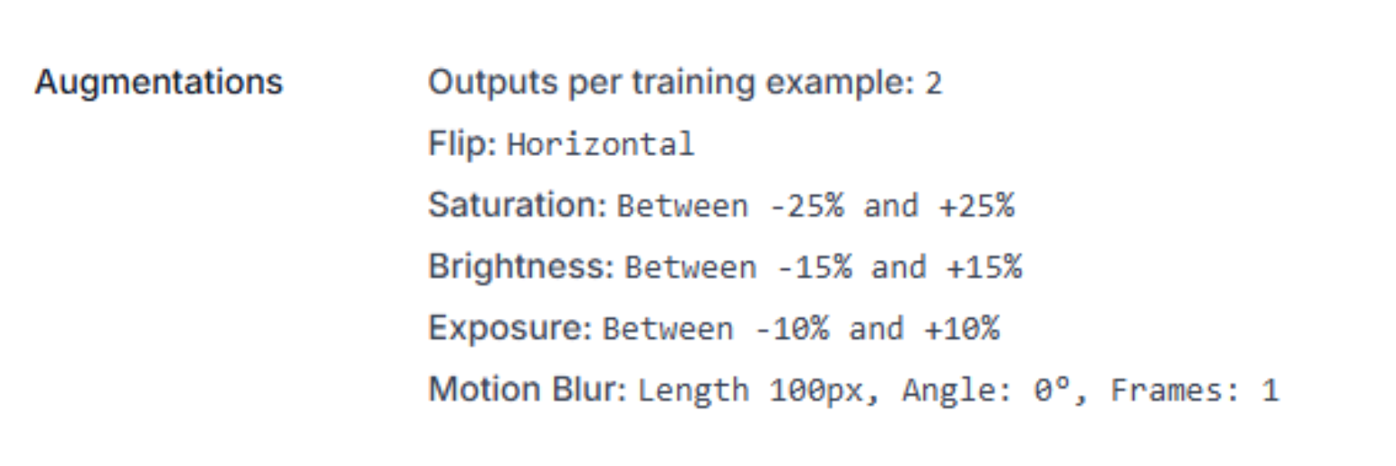
- Horizontal Flip: Doubles the training data by simulating plays moving in both directions.
- Saturation & Brightness (±25%): Prepares the model for high-noon sun glares and stadium floodlight variations.
- Motion Blur (100px): Essential for football, this helps the AI recognize players even when the camera pans rapidly during a long pass.
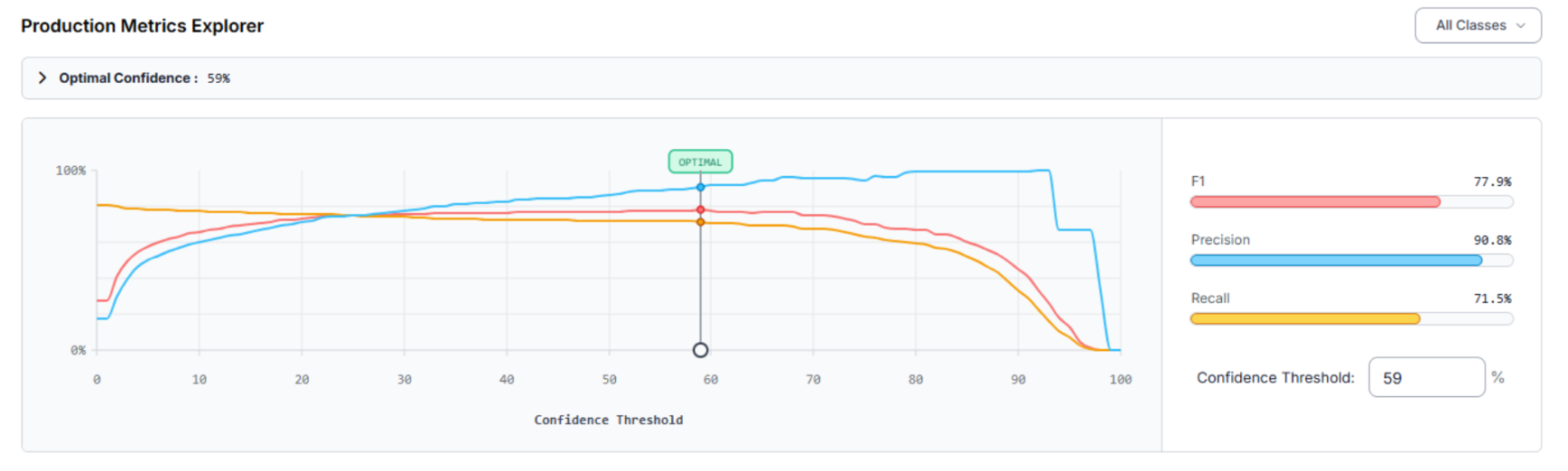
Step 7: Evaluate Model Performance
After training the RF-DETR model, we use the Production Metrics Explorer to audit the results. Our football detector achieved a mAP@50 of 74.8%. At an optimal confidence of 59%, the system reached an F1 Score of 77.9%.
- Precision (90.8%): When the system identifies a player, it is highly accurate, minimizing false positive detections.
- Recall (71.5%): The model captures the majority of the action, though dense scrums occasionally present challenges.
Optimization Roadmap:
- Differentiate Similar Classes: If classes are being confused, adding more varied samples of specific uniform patterns will sharpen the model’s discernment.
Expand Small Object Training: For wide shots where players appear small, implementing SAHI (Slicing Aided Hyper Inference) can significantly boost detection rates.
Building the Tracking Workflow
Now that the model is trained, we build the engine that runs the tracking. Follow these steps to build your tracking workflow in Roboflow. Here’s the one made in this article.
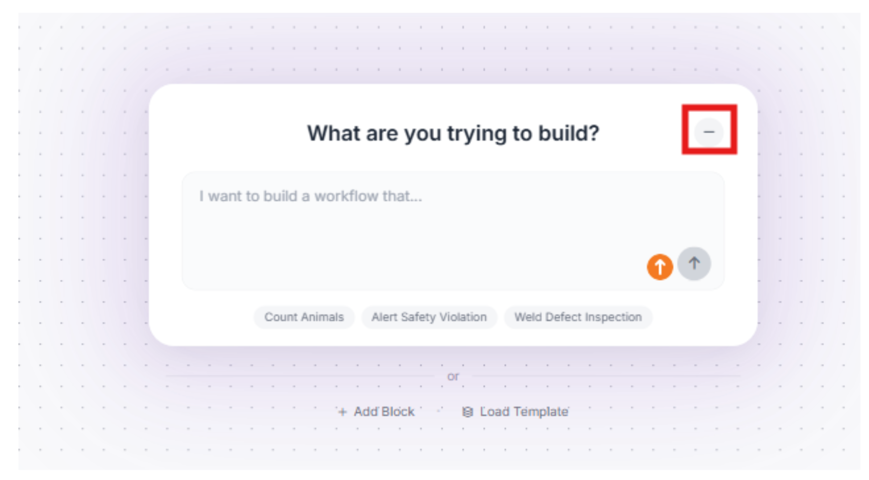
1. Initialize the Workflow
Navigate to the Workflows tab in the sidebar.
2. Minimize the Roboflow Agent
We won’t need the Roboflow agent for this, so we can minimize it.
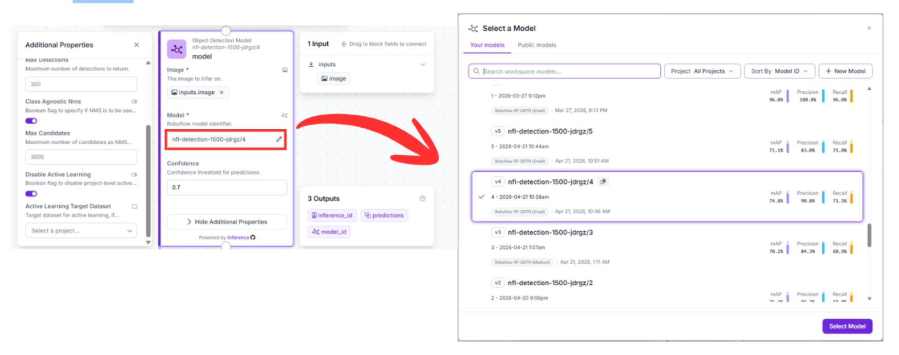
3. The Detection Block (RF-DETR)
Drag in the Object Detection Model block and connect it to your Input block.
- Configuration: Select your trained model (nfl-detection-1500-jdrgz/4).
- Function: This block analyzes the raw pixels and generates bounding boxes for every player.
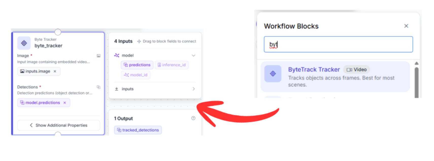
4. The Tracking Block (Byte Tracker)
Connect the output of your Detection block to the Byte Tracker block.
- Why this connection matters: The tracker requires the bounding box coordinates from the detector to maintain identity.
- Function: The Byte Tracker uses motion vectors to associate detections between frames. Even if a player leaves the frame for a split second or is obscured by a tackle, the tracker projects their position, ensuring identity persistence.
5. Visualization Blocks
To see the results, connect the tracker output to three successive visualization blocks. These blocks are chained because each adds a new layer of visual information to the previous step's output:
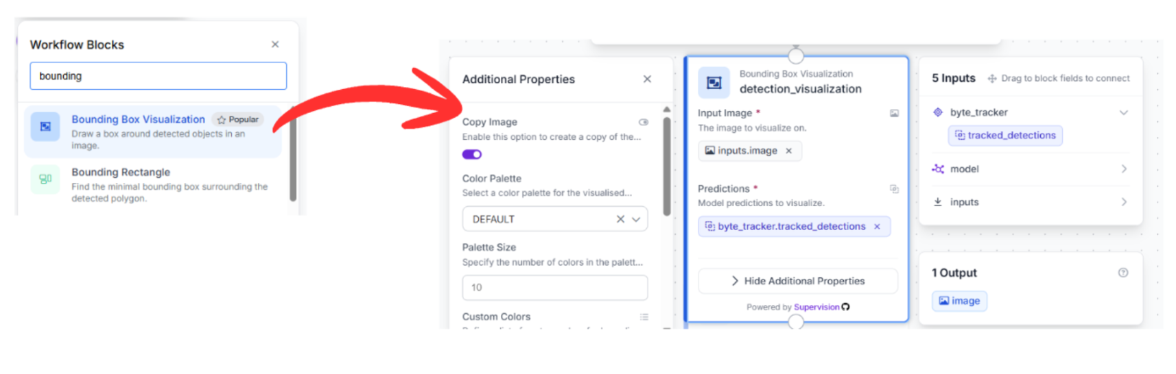
Bounding Box Visualization: Connect this to the Byte Tracker output. This draws the rectangles around the detected players.
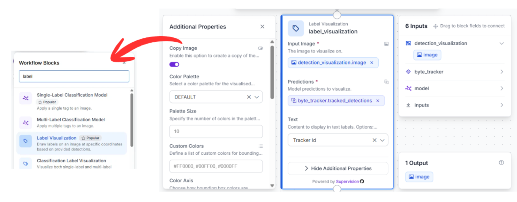
Label Visualization: Connect the previous visualizer to this block. This pulls the Track ID from the Byte Tracker and overlays the ID number onto the bounding box.
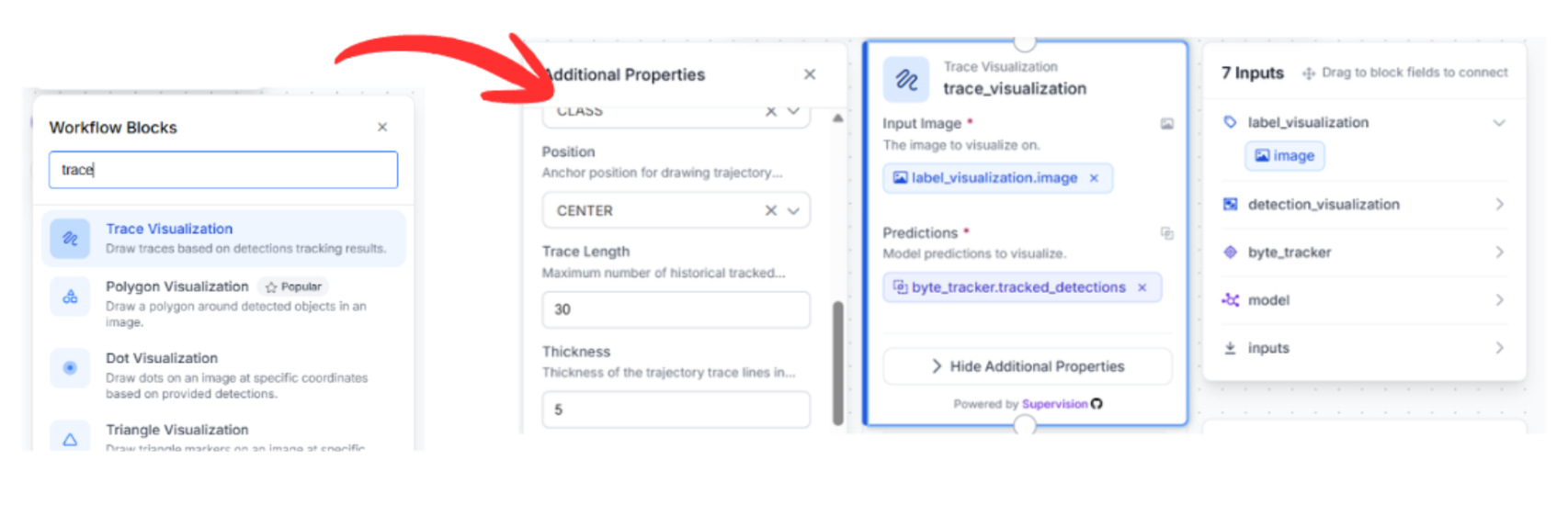
Trace Visualization: Finally, connect this to the label visualizer. This block maintains a history of the player's movement, drawing a "movement trail" behind each player’s ID.
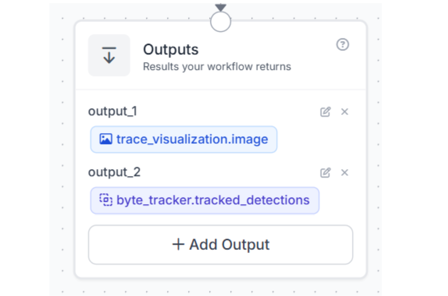
6. Outputs
Drag the Output block onto the canvas. Connect your final visualizer (Trace Visualization) to this block. Then choose to get outputs from the bytetracker and trace_visualization blocks. This will return the finished, tracked video stream containing both the bounding boxes and the movement history.
Test it:
Now that the workflow is assembled, it’s time to validate the system. By feeding raw game footage into our finalized workflow, we can observe the RF-DETR model and Byte Tracker in real-time execution.
Conclusion: Real-Time Player Tracking in American Football
True production efficiency is about transforming video into actionable intelligence. By splitting your architecture into a high-speed RF-DETR detector and a persistent ByteTrack memory, you create a system that does more than just see; it understands the flow of the game. This ensures every highlight reel is backed by accurate, searchable metadata.
Ready to modernize your broadcast pipeline? Sign up for a free Roboflow account and explore the latest sports datasets on Universe today.
Learn more about automating camera control.
Written by Aarnav Shah
How can I track football players in game footage?
To track football players in game or practice footage, you can build an automated computer vision pipeline using Roboflow combining a high-speed detection model with a persistent tracking algorithm. First, train RF-DETR (Small), a lightweight, low-latency model, on domain-specific football footage so it can instantly detect players and generate accurate bounding boxes. Next, route those detections through the tracking system ByteTracker, which uses motion vectors to maintain player identities and track IDs across consecutive frames, even during dense scrums or when players are briefly obscured. Finally, run the output through visualization tools to overlay bounding boxes, player IDs, and movement trails directly onto the live broadcast video.
Cite this Post
Use the following entry to cite this post in your research:
Contributing Writer. (Apr 24, 2026). Real-Time Football Analytics: Building a Player Tracker with RF-DETR and ByteTrack. Roboflow Blog: https://blog.roboflow.com/american-football-player-tracker/