
Counting salmon passing through a fish ladder viewing window is currently done by trained human observers, but object detection models can automate and scale that work. Data scientist Jamie Shaffer trained a computer vision model on fish ladder footage, reaching a meaningful mAP@0.5 on a dataset where image quality varied considerably, showing that imperfect images do not prevent a working prototype. Remaining challenges include tracking individual fish across frames and handling erratic swimming behavior that differs from a static counting scenario.
The below is a guest post from Jamie Shaffer, a data scientist based in Washington state. She is open to new opportunities, particularly leveraging deep learning to environmental issues.
Living in the Pacific Northwest, the intertwined issues of salmon survival and river flow are frequently in the news, and the data we have on our salmon populations is a key piece in the conversation.
0:00/1×
I wanted to see if deep learning — object detection in particular — was up to the challenge of assisting with the real world problem of counting fish seen passing through a fish ladder.
The answer is yes, and there are enough free or open source tools available to accomplish all aspects of the task.
This approach can be used to count other objects as well. If you have an idea and a place to grab a few images, you can use this walkthrough to help you get your own computer vision models running.
Step 1: An intriguing issue
The Pacific Northwest is home to many species of salmon whose lives follow a predictable pattern: hatch in fresh water, migrate to the ocean for the majority of their lives, and then migrate back upstream to their original fresh water hatch sites before they spawn and then die.
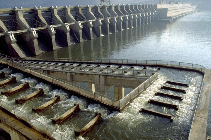
Salmon aren’t the only ones using the rivers though. Hydroelectric dams dot our rivers for hundreds of miles, potentially preventing the upstream migration. To solve this, our dams are all built with something called a ‘fish ladder.’ These constructions allow fish to jump upstream in short segments much as they would in an openly flowing river.
Salmon ladders with viewing windows also provide us with the means to witness this migration and to collect data. Data on the number of salmon returning upstream can then be used to determine the length of the fishing season, set limits on fish per day, adjust the flow at the dam, and help us understand how well we’re doing in this balancing act.
Counting fish is currently performed by trained experts either as real time counts or by reviewing video recordings. Given how labor intensive this is, an assist from an expert tool could provide a nice boost to increase the amount of data taken, the speed at which it is available, or the number of locations where the data is recorded.
Step 2: Images and pre-processing
Whichever project you choose, you’ll need to start with data. Don’t be dissuaded if you can’t start with ideal data; there’s still plenty to learn. I started with web scraped images of vacation photos taken at fish ladders. The images contained a variety of locations, lighting conditions, silhouettes of children, and possible post-production modifications. The images were so difficult to work with that all I could really label was what constituted a “fish”! I ran the rest of this flow with just that and worked out quite a few bugs, so remember that you can start simple. Once I had a sense of what I needed, I found my way to some better images recorded on a video.
For the images in video format, I used the free VLC Media Player tool to run the video and extract 300+ frames. I selected 317 images including 15 images with no fish at all.
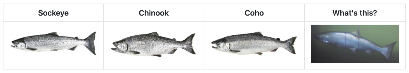
To prepare these images for deep learning, I also needed to associate a correctly labeled box with each object to be detected. Trained experts label fish by species, mature vs. juvenile, and hatchery vs. wild.
Without fish identification expertise, it was still possible to create 3 classes:
- ‘adipose’ for fish having an intact and visible adipose fin
- ‘no_adipose’ for fish having no adipose fin
- ‘unknown’ for fish only partially in the viewing window, or whose adipose fin region is obscured by another fish or artifact
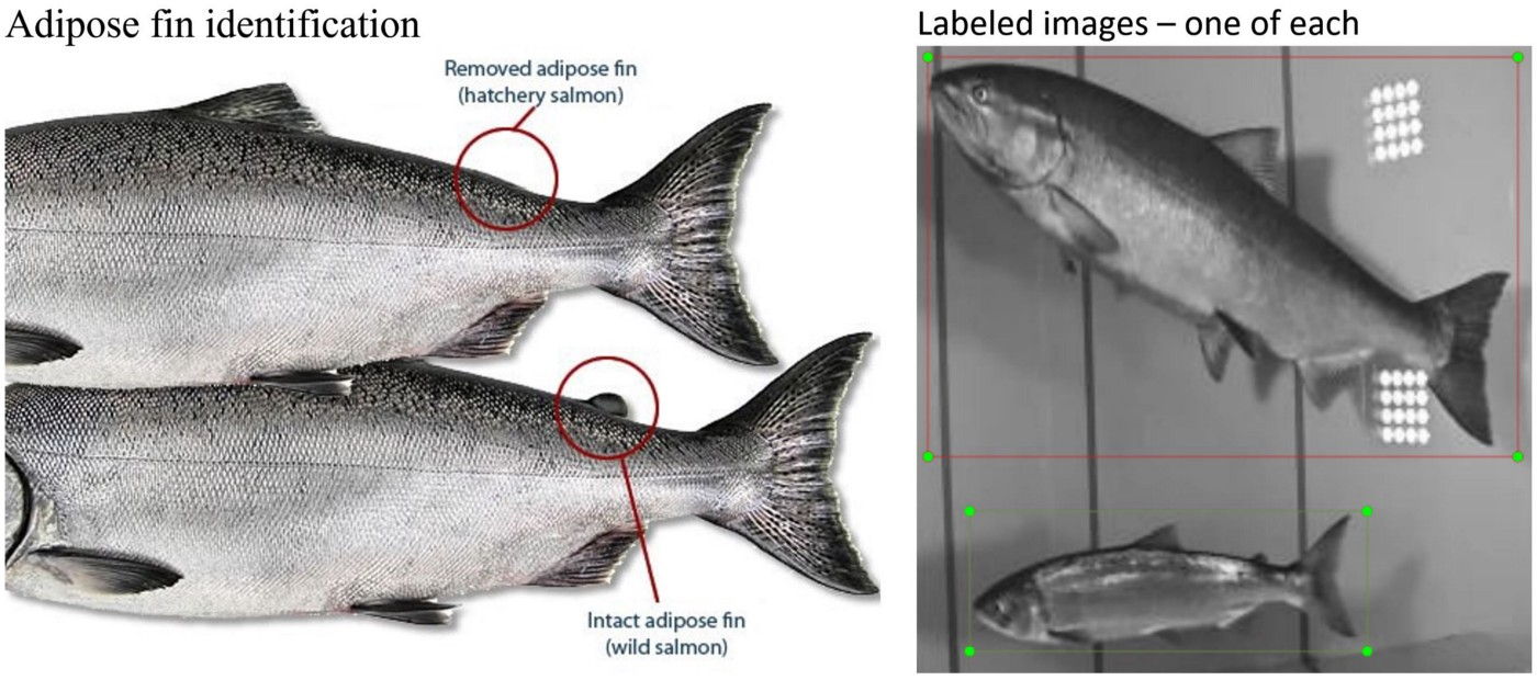
The free tool LabelImg worked well and I had my 317 fish images boxed and labeled in an afternoon.
One of the reasons I knew thatI could get a model working with only 300 or so images was the idea of augmentation. Augmentation takes the originals and constructs variations so that the model is exposed to a variety of changes such as lighting and orientation. With classification, this is easily performed with a few python libraries, but for object detection, the label boxes also need to be transformed if the image is flipped or rotated.
Rather than do these transforms by hand, I leveraged the free tools at Roboflow. I uploaded my images and my label file, selected options to create additional images with random amounts of blur, changes in brightness, and horizontal flip. After this step, I had 951 training images.
Step 3: Select and train a model
While it’s possible to build a home-grown object detection model, I opted to start with a known model for my project as a baseline before doing any tailoring. All of this can be done from the model library at Roboflow, and it’s possible to try out more than one.
“You Only Look Once”. YOLO is a popular object detection machine learning model introduced in 2015 by a group of researchers at the University of Washington. Rather than pass an image classifier multiple times over an image to see if there was, say, a dog at the upper left, or maybe at the upper right, this new approach replaced the final layers of an image classifier with additional convolutional layers that allowed it to find all instances in one pass. The immediate improvement in speed was a major leap forward for computer vision and object detection. Since the original paper, the model has been improved several times and a new model built on this earlier foundation was released in June 2020 as YOLO v5. See the repository at https://github.com/ultralytics/yolov5 for more details on the model.
Given the popularity, speed, and accuracy of YOLO, and the ease of leveraging the tools at Roboflow, trying out the YOLO v5 model was an obvious choice. Starting with a Google Colaboratory template that configured the environment and built the model, I customized this by uploading a new training set, experimenting with various epochs and thresholds.
Step 4: Explore model results
The results were impressive and informative.
Impressive — the YOLO v5 model trained for 500 epochs in about an hour on the 900+ images, ran inference (prediction) on a new image in about 12 msec, and achieved mAP@0.5 of about 70%.
Individually viewing and rating the model’s success on test images would be a bit of a chore, though, so this is where the mAP@0.5 metric is valuable.
mAP@0.5
This metric contains two pieces. First, ‘mAP’ indicates the mean Average Precision or correctness of each of the 3 labels taking into account all labels. Second, ‘@0.5’ sets a threshold for how much of the predicted fish bounding box overlaps the original annotation. This second part is a key metric in object detection; it prevents the model from getting credit for guessing the correct fish but drawing a box around some other artifact (like a shadow) instead of an actual fish.
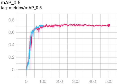
This model achieved a mAP@0.5 of 70% —but is that good or bad? For some applications, it’s more than enough. In this particular application, there’s more to it than the label assigned to a single image, and ideally the results of a full solution need to be compared to an estimated error in our current fish counting methods.
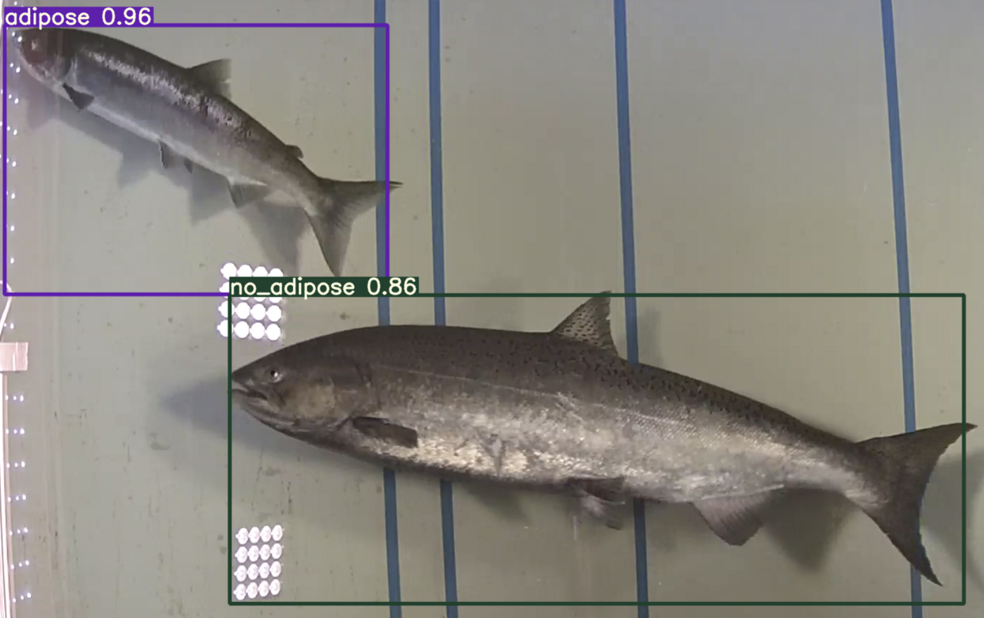
Informative — altered lighting conditions, shadows, and crowded conditions can result in both under and over counts. In the image below, the confidence threshold was intentionally set low at 0.4 to expose corner cases or images that provide a challenge for the model. Keep in mind that the goal is to see if we’re ready to use this for a real-life challenge, and that means looking for problems!
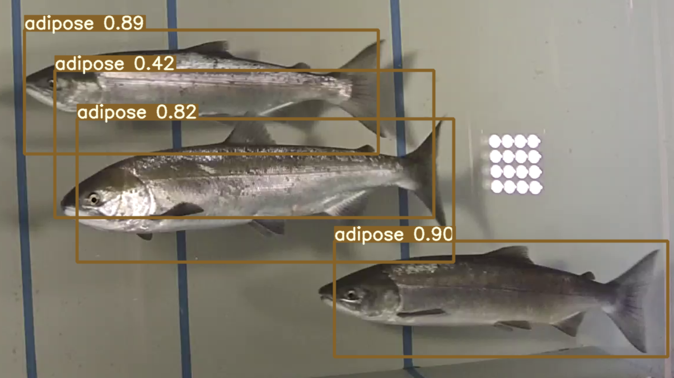
In the actual application, when the objects are tracked from one frame of video to the next, shadows often move and the label disappears. This next level of challenge will be to address the object tracking from frame to frame so that there is exactly 1 count for each fish, no matter how much time it remains in the viewing window.
Step 5: Consider next steps
Now the most important step — what did I learn?
- Images with excellent lighting are required
- Viewing window height and width are not critical, but the depth needs to be carefully selected to reduce the number of fish that can obscure other fish
- Correct species labels are required for training a model to separate sockeye, chinook, and coho in addition to other species. Not being a fish identification expert, there is the possibility that I mistook a scar for a small adipose fin. Correcting mislabeled images is another way to improve the model.
- Salmon swimming upstream in a fish ladder pause to rest for varying amounts of time. In some cases, they will swim slowly and maintain position, and at other times they will slow to the point that they drift backward with the current. This adds an additional level of complexity that will require an advanced system to track objects (fish) from one video frame to the next.
Most importantly, while the metrics above are from the better images, most of this learning happened on the first set of images, underscoring the point that excellent images are not required to make progress in trying out a project with deep learning and object detection. In other words, not finding ideal images shouldn’t hold you up from getting started!
Conclusion
Based on the project so far, I think it’s fair to say that machine learning / AI / deep learning are ready to be taken out of the lab and applied to real world projects.
This is good news — as an indicator species, salmon help us assess the health of our environment. Accurate and timely fish counts are critical to ensuring their survival, and ours.
Cite this Post
Use the following entry to cite this post in your research:
Joseph Nelson. (Aug 23, 2020). Using Computer Vision to Count Fish Populations (and Monitor Environmental Health). Roboflow Blog: https://blog.roboflow.com/using-computer-vision-to-count-fish-populations/