
Standard object detection models lose accuracy on small targets because the relevant features occupy too few pixels at full image resolution. Slicing Aided Hyper Inference (SAHI) addresses this by dividing a large image into overlapping tiles, running inference on each tile independently, then merging the results. This guide shows how to implement SAHI inside Roboflow Workflows using the Image Slicer block paired with any object detection model and the Detections Stitch block, producing a workflow that can be deployed to the Roboflow cloud or on dedicated hardware for video and RTSP stream inference.
When working on a computer vision project that involves detecting small objects, using the SAHI technique can help improve detection accuracy.
Slicing Aided Hyper Inference (SAHI) is a technique where you split a large image up into smaller images, run inference on each smaller image individually, then stitch together the results.
Here is an example of an image processed without and with SAHI:
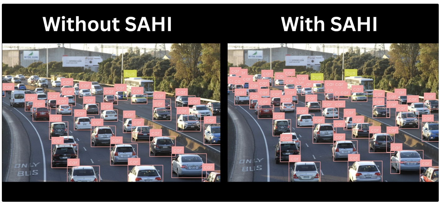
SAHI-based small object detection detects substantially more objects than using an object detection model alone.
With Roboflow Workflows, you can build a system that detects small objects using the SAHI technique with a variety of public or custom-trained models in just a few minutes.
In this guide, we will build a small object detection workflow using the Image Slicer block in Roboflow Workflows to implement SAHI.
Without further ado, let’s start building the workflow!
Small Object Detection with Image Slicer
Roboflow Workflows has a block called Image Slicer that slices an input image into smaller pieces. These image segments can be run individually through an object detection model. The detections can then be stitched back together.
The workflow we will build will have the following steps:
- Accept an input image.
- Slice the image using the Image Slicer.
- Run an object detection model.
- Stitch the results back together using the Detections Stitch block.
- Use visualization blocks (e.g., bounding boxes, labels) to visualize the results.
Step #1: Create a Workflow
To get started, first create a free Roboflow account. Then, navigate to the Roboflow dashboard and click the Workflows tab in the left sidebar. This will take you to the Workflows homepage, as shown below, where you can create a workflow.
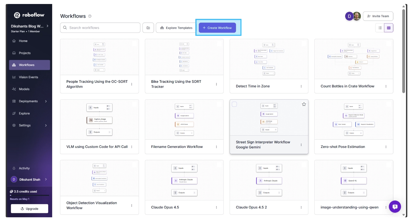
Click "Create Workflow" to create your workflow. You will be taken to the Workflows editor, where you can build and configure the workflow.
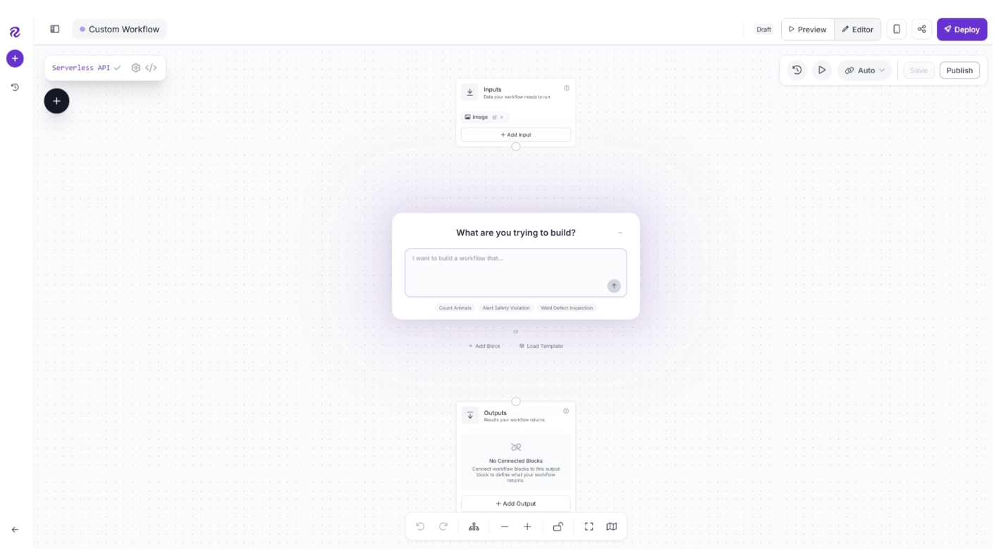
By default, you will see two blocks: Inputs and Outputs, along with an AI Assistant pop-up that can help generate workflows from prompts. You can minimize the pop-up for now and focus on building the workflow step by step.
An example prompt you can use to generate the workflow described in this guide is shown below. While you may need to adjust some settings to better fit your specific use case, it provides a solid starting point.
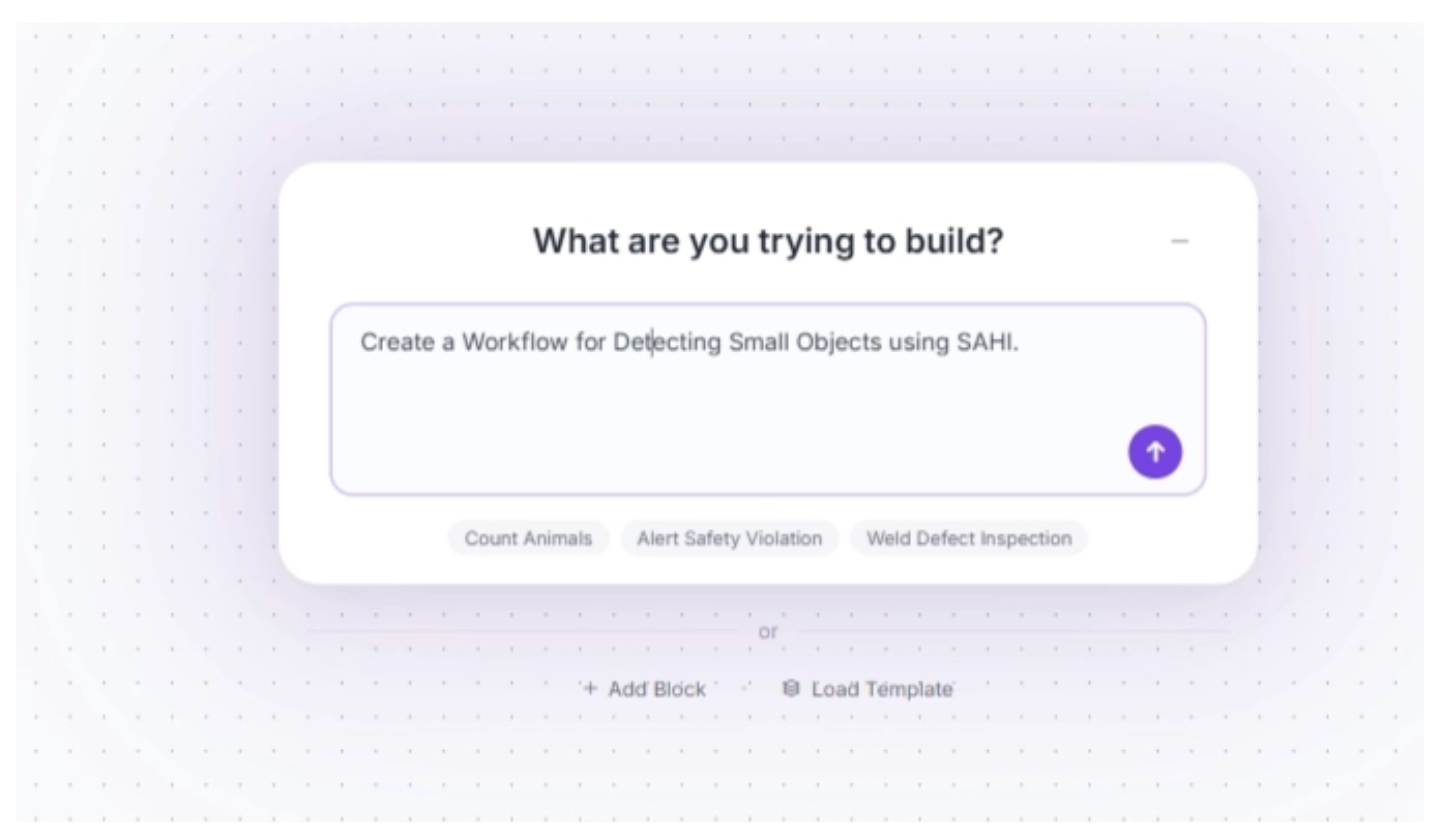
You can also rename your workflow by clicking the ⚙️ icon in the top-left corner.
Step #2: Add Image Slicer
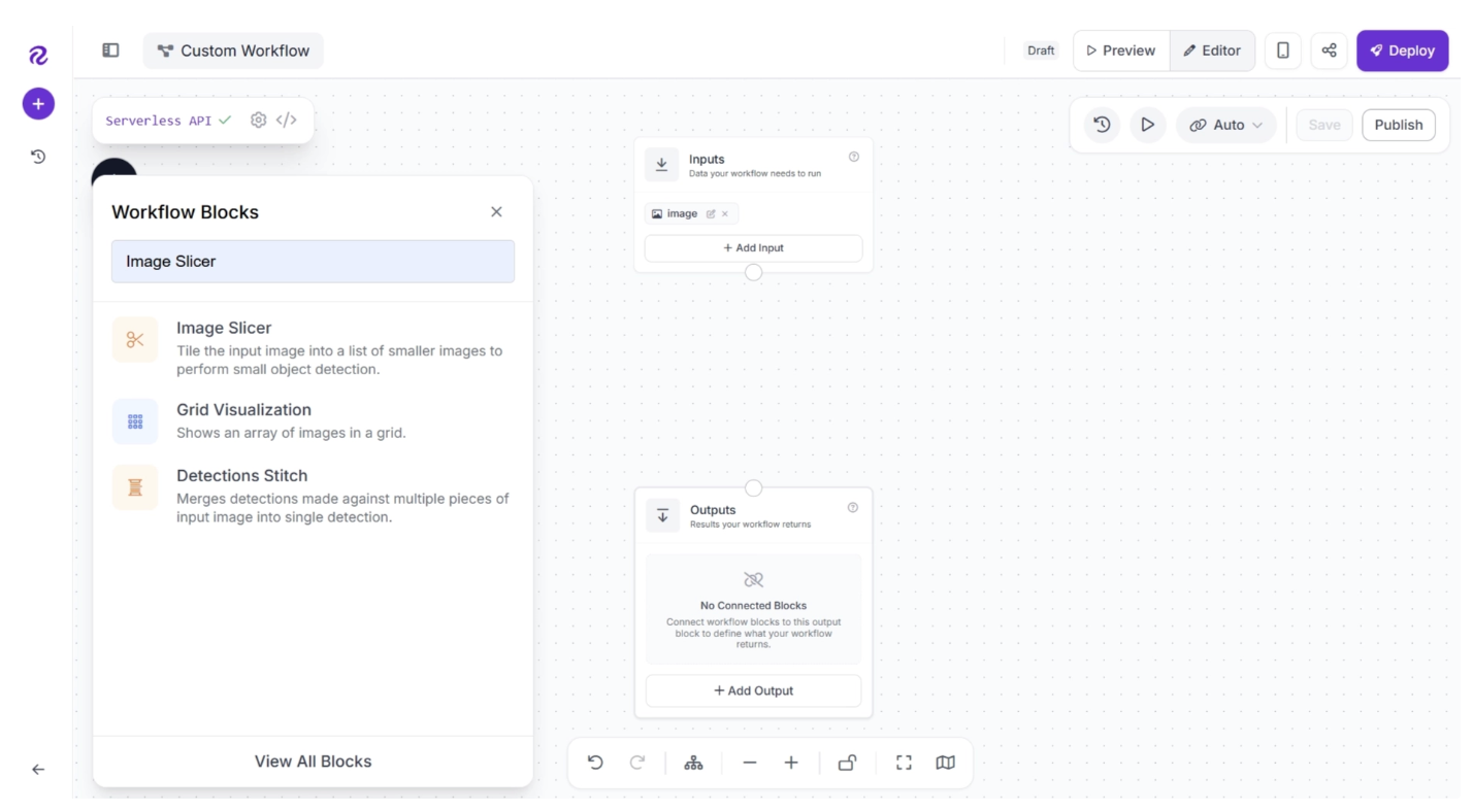
With a basic Inputs-Outputs workflow ready, we can start using the Image Slicer. To add it, click the “+” button in the top-left corner of the workflow editor. A menu of available blocks will appear, as shown below. Search for “Image Slicer” and insert it into your workflow.
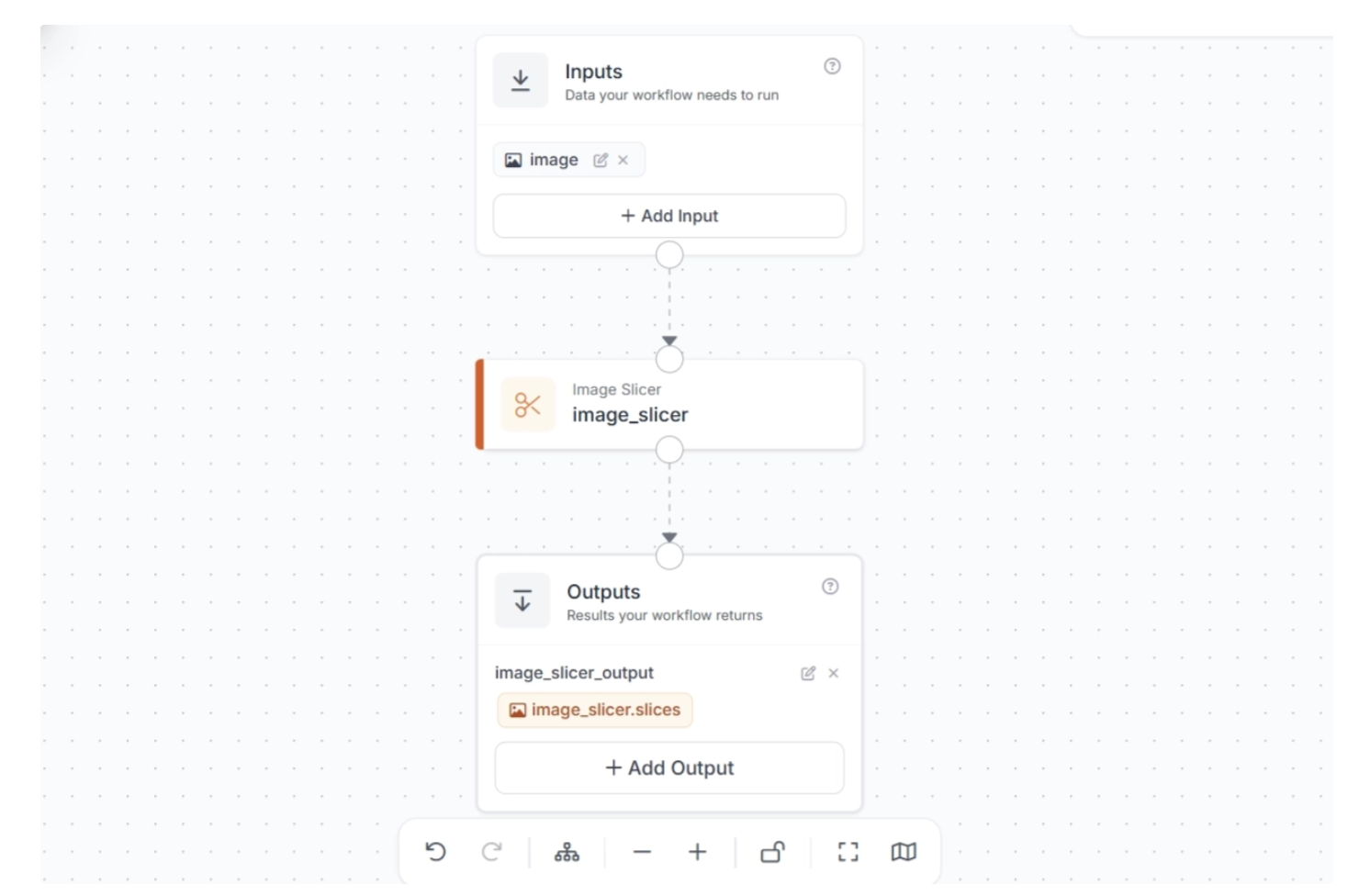
Once added, the workflow should be automatically configured as shown below.
Note: Make sure to publish the workflow after adding the blocks to save your changes.
Step #3: Add a Model
Next, we need to add a model that we want to use to run inference on our image slices. For this, we use an Object Detection block.
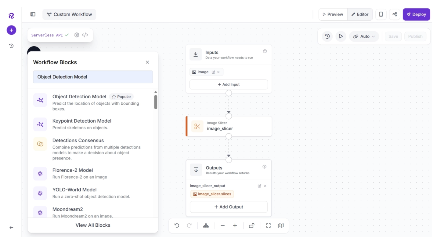
To add it, click the “+” button in the top-left corner of the workflow editor. A menu of available blocks will appear, as shown below. Search for “Object Detection Model” and insert it into your workflow.
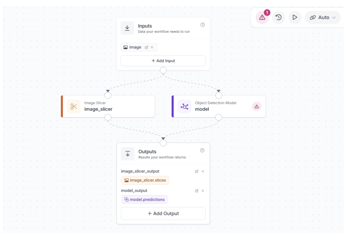
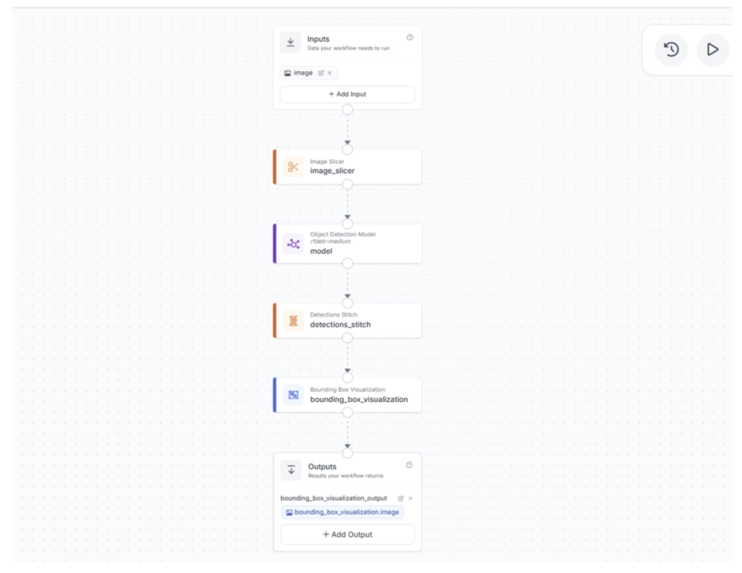
Once added, your workflow will look like this:
We want to feed the image slices produced by the Image Slicer to the model. To do this, connect the Image Slicer block to the Object Detection Model block. This ensures that the image slices flow into the model for inference. Also, delete the unnecessary connection from the Image Slicer block to the Outputs block.
After connecting the blocks, click Auto Layout (to the left of the zoom controls at the bottom) to neatly organize the workflow in the editor. Your workflow should now look like this:
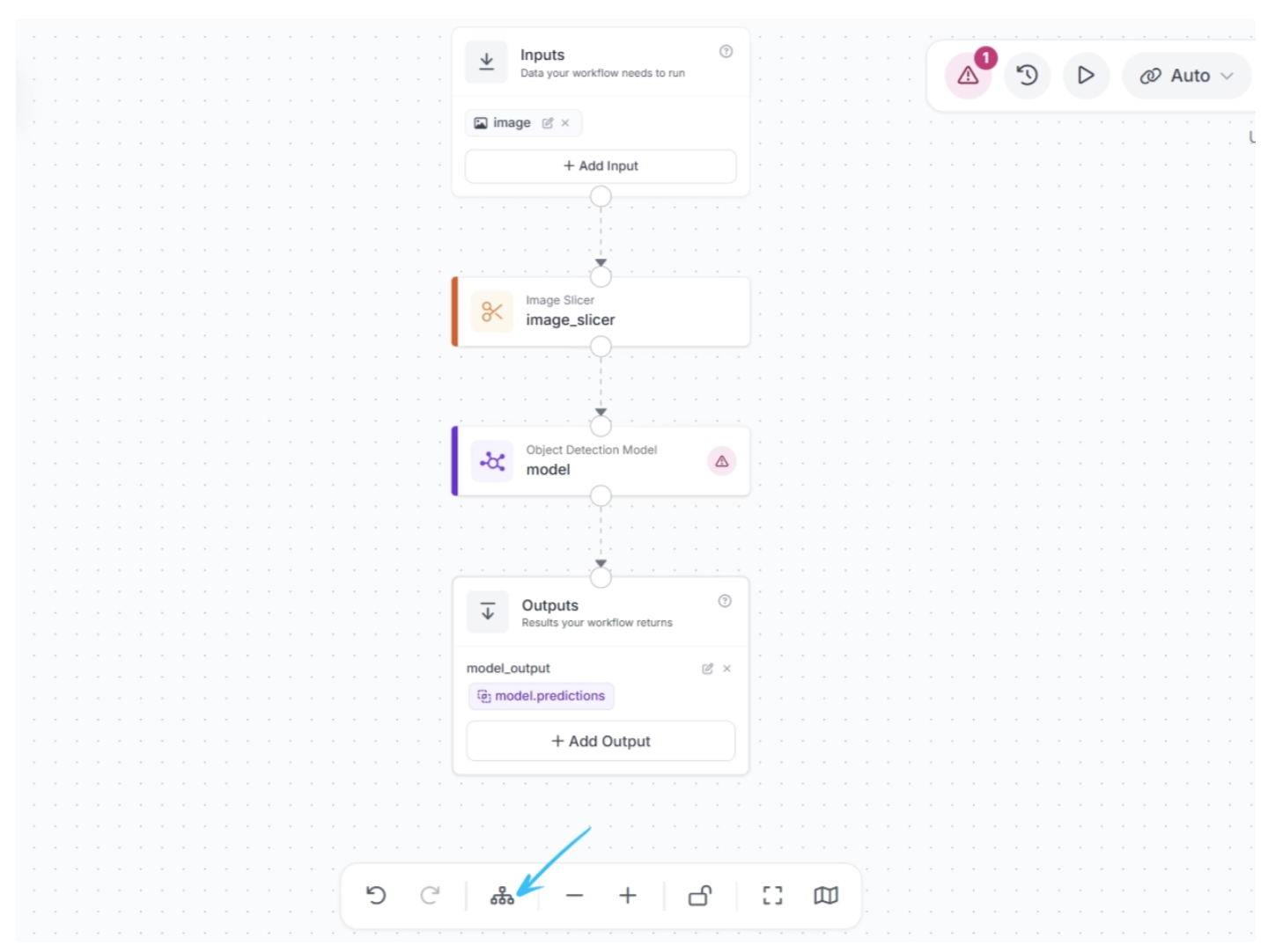
Note: When a connection is made between two blocks, the downstream block receives the output from all upstream blocks, which can then be used as inputs for its parameters.
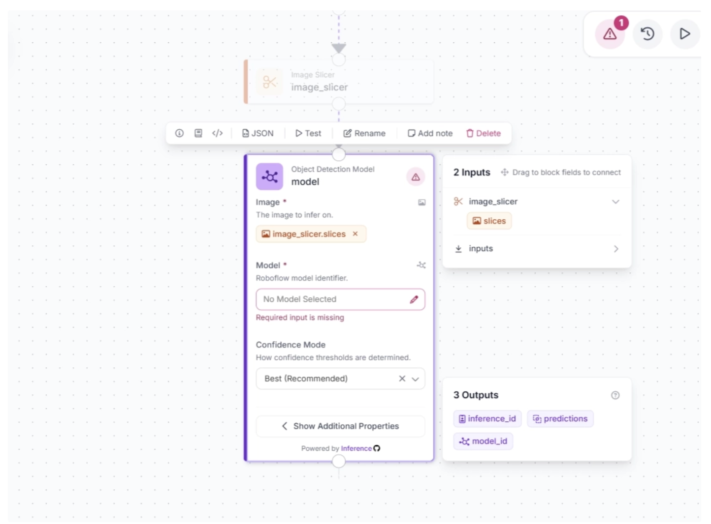
Make sure the Object Detection Model block is configured to accept the image slices from the Image Slicer block, as shown below.
Now, configure the detection model for inference in the Object Detection model block. You can use any model in your Roboflow workspace or any model hosted on Roboflow Universe.
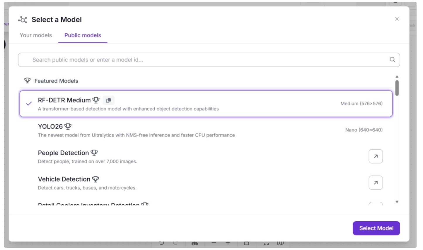
For this guide, we are going to use RF-DETR, Roboflow’s real-time transformer-based object detection model. RF-DETR was trained on the Microsoft COCO dataset and can identify a variety of common objects, including cars, cell phones, and people.
To configure the detection model, select the Object Detection Model block to expand its parameters, then click the ✏️ icon under the Model parameter. This will open a model selection pop-up, as shown below. From there, select the RF-DETR Medium variant.
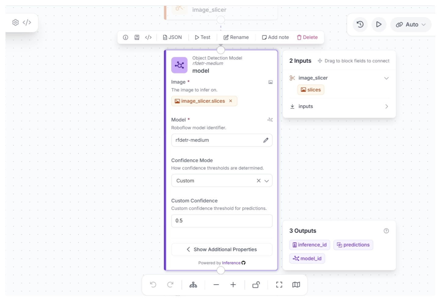
Once the model is selected, you can configure the confidence score. For this use case, set the confidence mode to “Custom” and set the Custom Confidence to 0.5, as shown below.
Step #4: Stitch Detections
So far, our workflow slices an input image and runs inference on each slice. Now, we need to combine the detections to complete our use of the SAHI technique for small object detection.
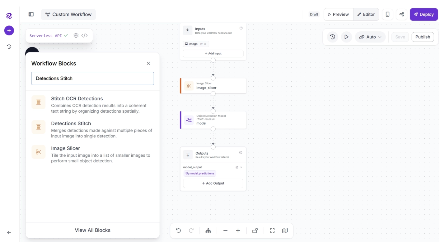
You can use the Detections Stitch block to combine detections. To add this block, click the “+” button in the top-left corner of the workflow editor. A pop-up menu with workflow blocks will appear. From there, search for “Detections Stich” and select it to insert it into your workflow:
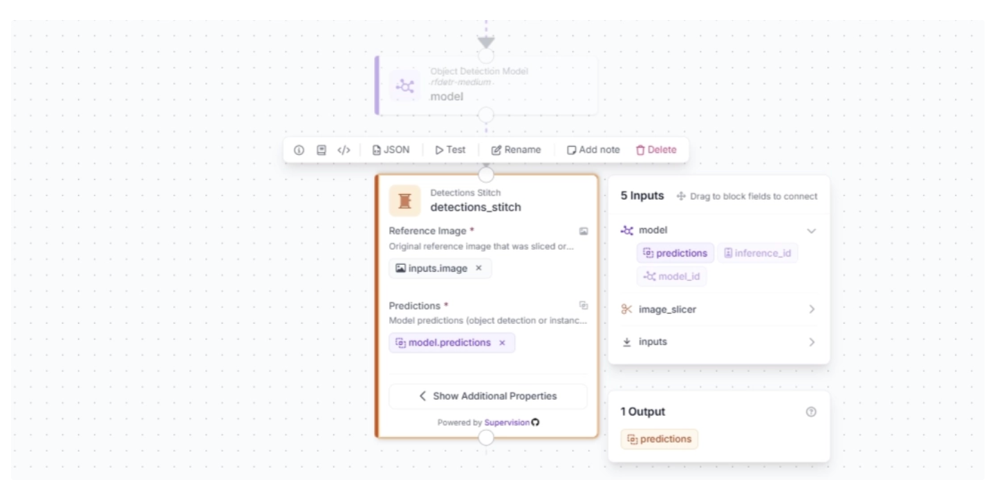
Make sure to set the Reference Image input to the original input image, and the Predictions input to the model predictions from the Object Detection Model block.
Step #5: Add a Visualizer
Now we can visualize the detections from the vision model. Roboflow Workflows supports several visualizers that display detections from vision models.
For this guide, we will use two visualizers:
- A bounding box visualizer, which will draw bounding boxes from our model, and;
- A label visualizer, which will add prediction labels on top of the bounding boxes.
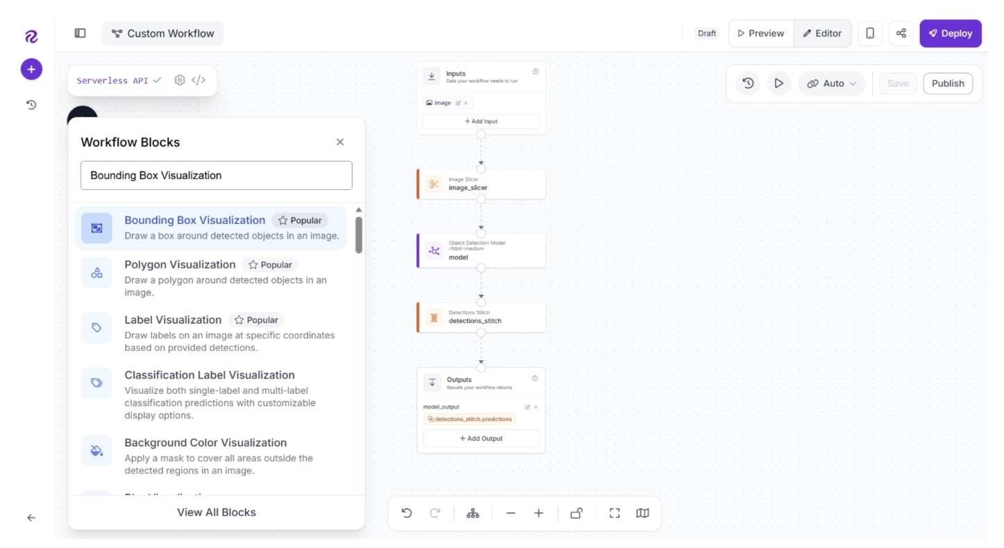
To add Bounding Box Visualization block, click the “+” button in the top-left corner of the workflow editor. A pop-up menu with workflow blocks will appear. From there, search for “Bounding Box Visualization” and select it to insert it into your workflow.
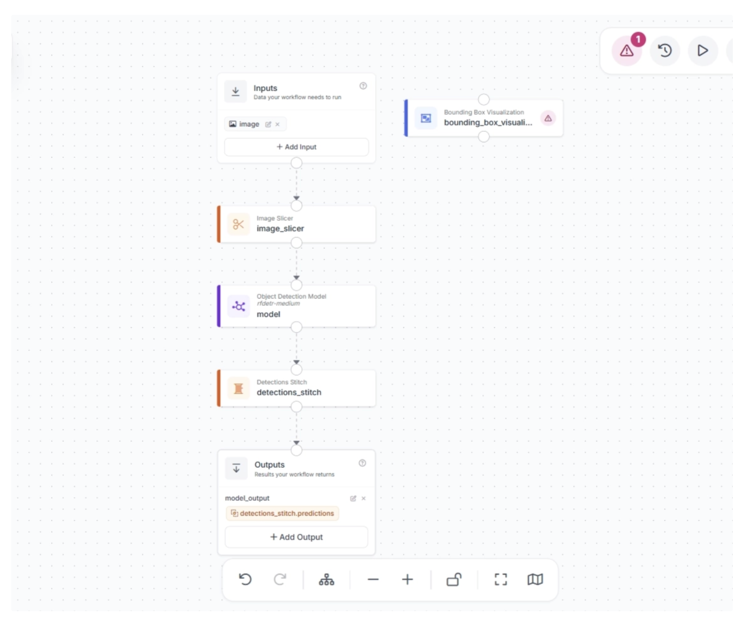
When added, the workflow editor will appear as shown below. The bounding box block is disconnected from the workflow.
You need to connect the Detection Stitch block to the Bounding Box Visualization block to use it in the workflow, as shown below.
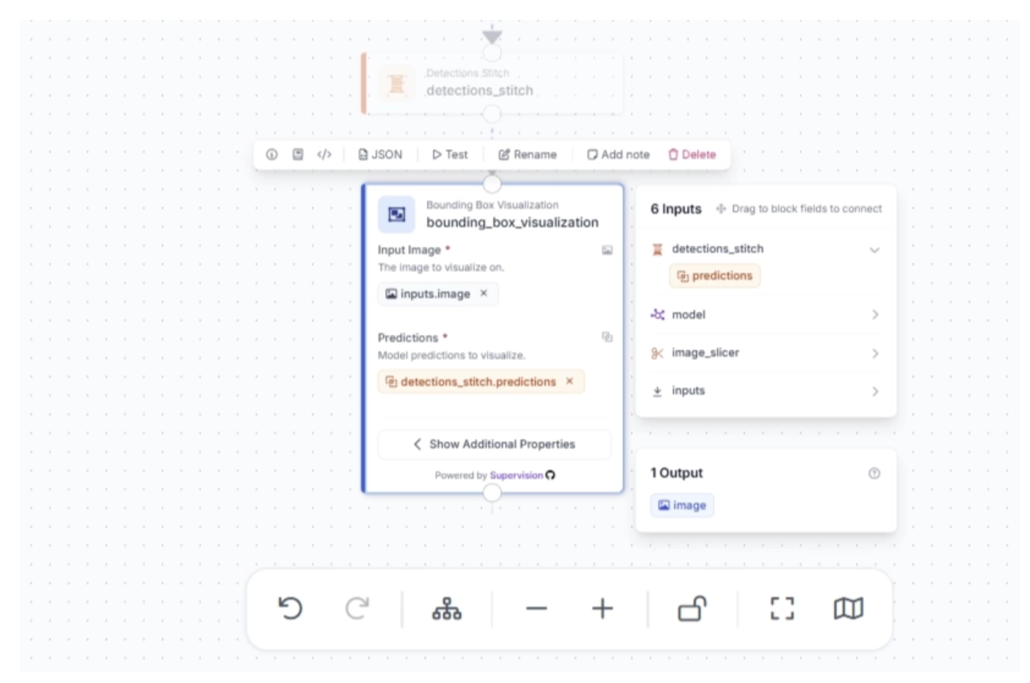
Make sure that the Bounding Box block is configured as shown below, where it uses detections from the Detections Stitch block and the original input image.
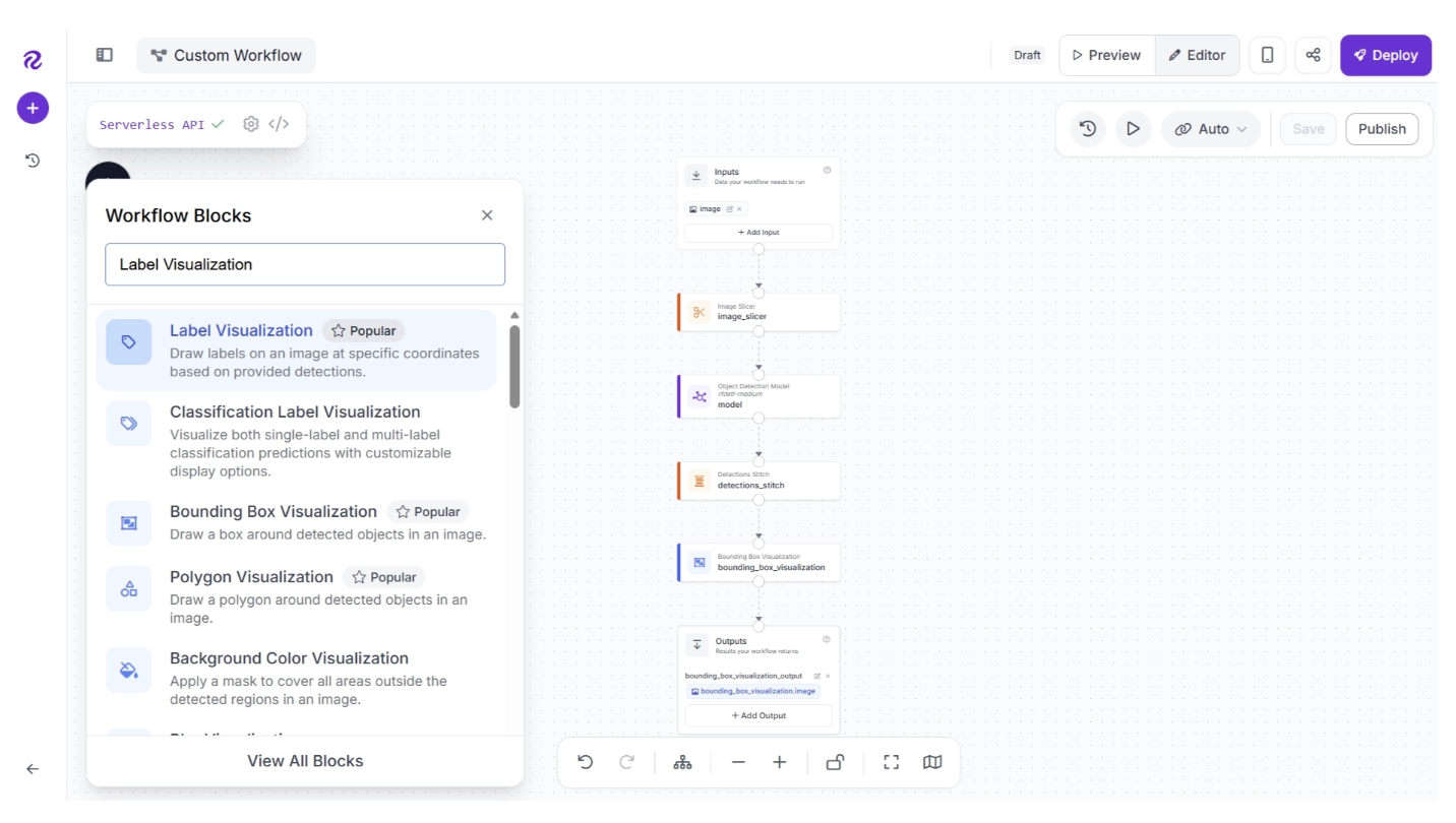
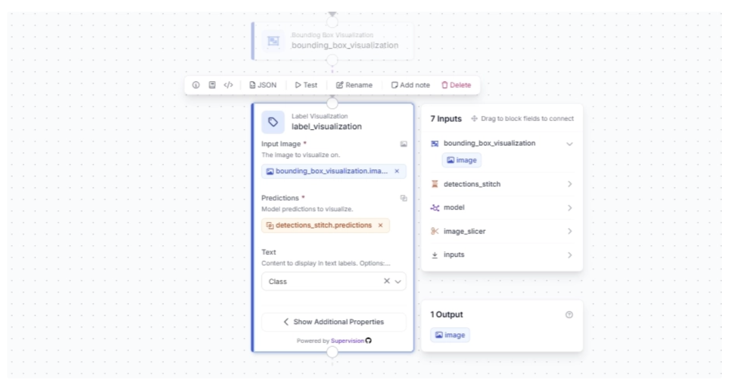
Now to add Label Visualization block, click the “+” button in the top-left corner of the workflow editor. A pop-up menu with workflow blocks will appear. From there, search for “Label Visualization” and select it to insert it into your workflow.
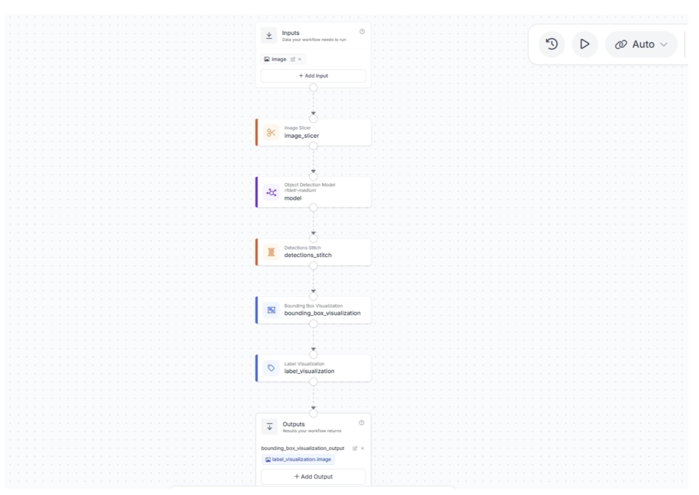
Once added, create a connection from the Bounding Box Visualization block to the Label Visualization block. Your workflow should looks like the one shown below:
Make sure the Label Visualization block uses the Bounding Box visualized image as input and the predictions from the Detections Stitch block. Also, set the text to display as “Class”; this will show the name of the detected object. All of this is configured as shown below.
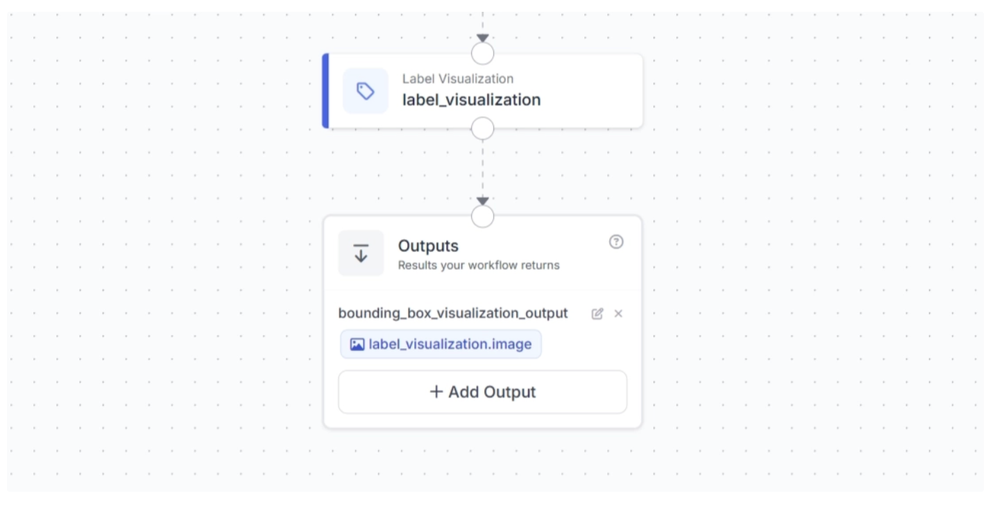
Now configure the output of the workflow to return the label-visualized image, as shown below.
We now have all the blocks we need to detect small objects with our workflow and visualize the results.
Step #6: Test the Workflow
Your final Workflow should look like this:
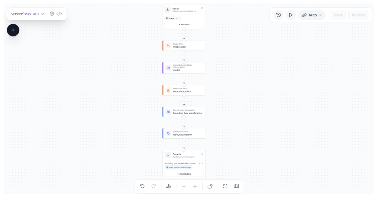
This Workflow:
- Accepts an input image.
- Slices the image.
- Runs an object detection model on each slice.
- Stitches the detections back together.
- Visualizes the detections with bounding boxes and labels.
To test the workflow, click “Run” at the top of the Workflows editor, as highlighted below:
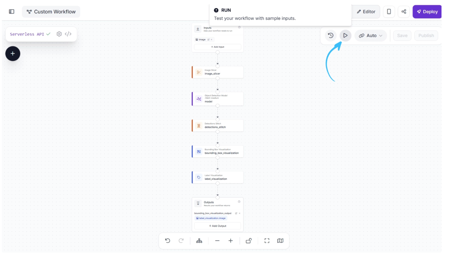
Then, drag in the image you want to use and click “Run” to execute the workflow.
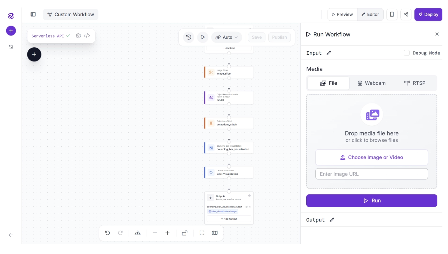
The result from the Workflow will appear on the right panel. Click "Visual" on the right panel to see detections from the system.
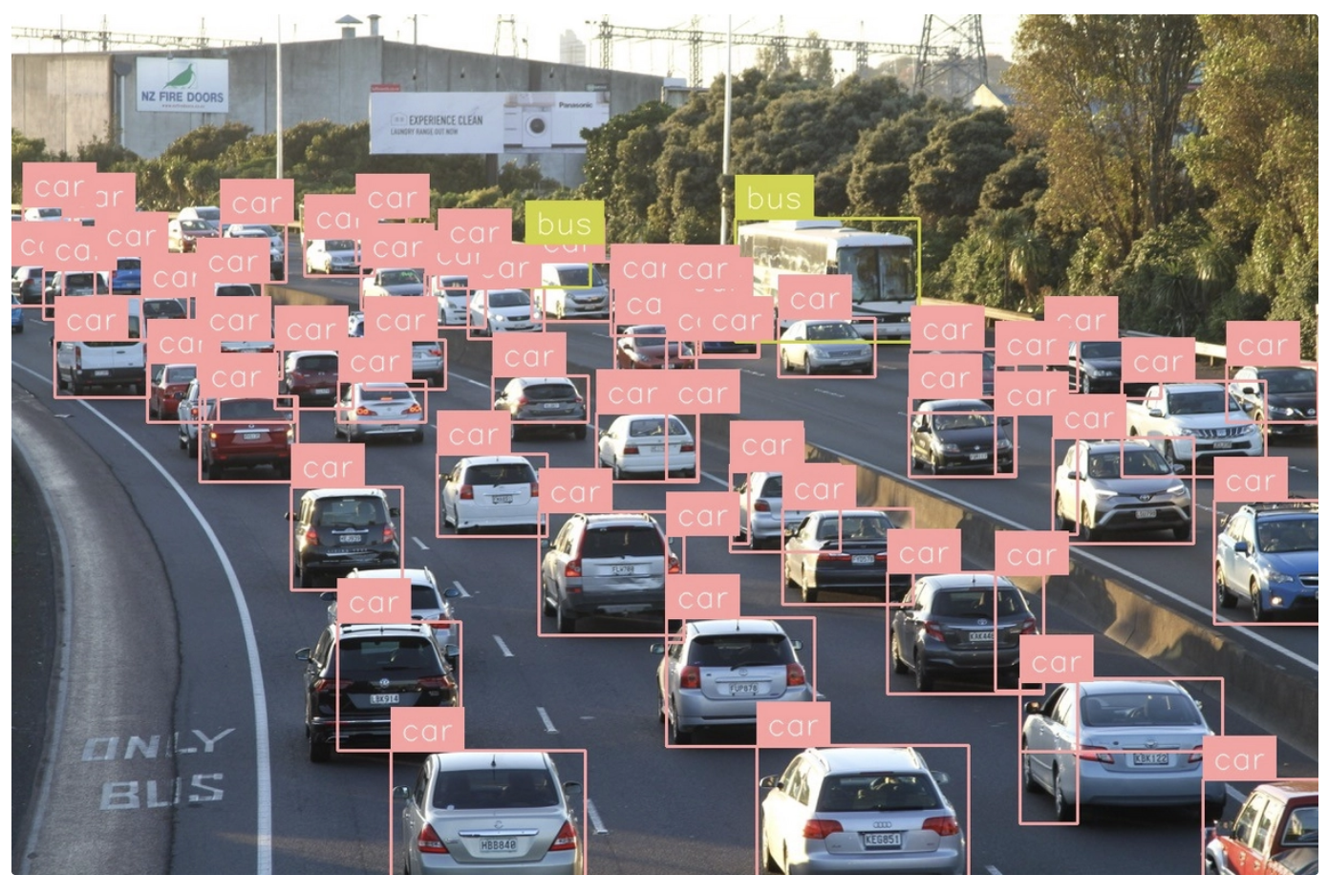
Here is the result of our workflow that uses the Image Slicer.
For reference, here is the result without Image Slicer, computed using only the object detection block and visualizers, without the Image Slicer.
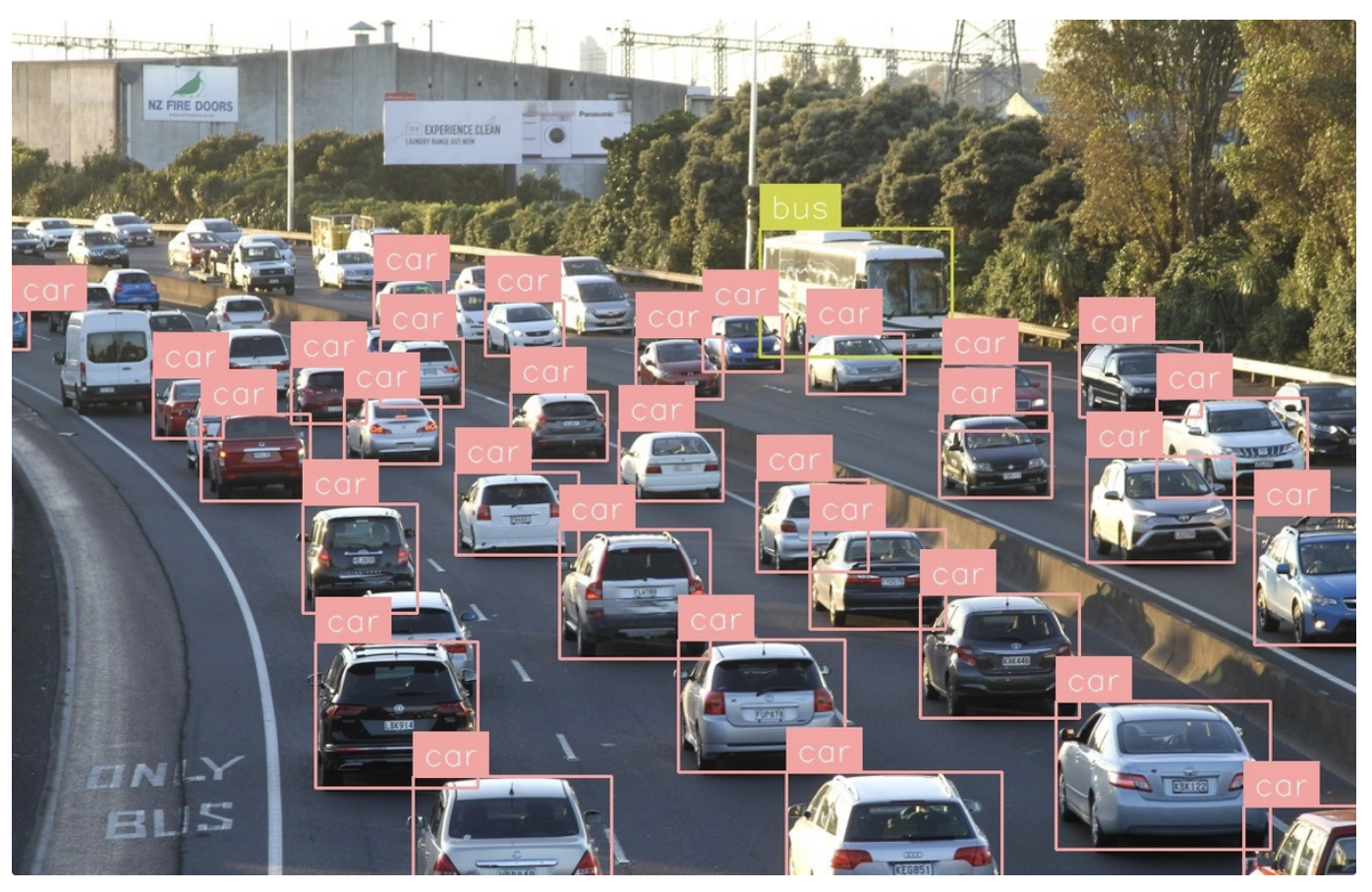
Our SAHI-based small object detection Workflow detects substantially more objects than the same Workflow that only uses an object detection model.
Deploy Your Workflow
You can deploy a Workflow in three ways:
- To the Roboflow cloud using the Roboflow API;
- On a Dedicated Deployment server hosted by Roboflow and provisioned exclusively for your use, or;
- On your own hardware.
The Workflows deployment documentation walks through exactly how to deploy Workflows using the various methods above.
Deploying to the cloud is ideal if you need an API to run your Workflows without having to manage your own hardware. With that said, for use cases where reducing latency is critical, we recommend deploying on your own hardware.
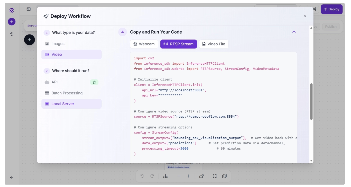
If you deploy your model in the Roboflow cloud, you can run inference on images. If you deploy on a Dedicated Deployment or your own hardware, you can run inference on images, videos, webcam feeds, and RTSP streams.
To deploy a Workflow, click “Deploy” in the Workflow Editor in your Roboflow Workspace. A window will then open with information on how to deploy your Workflow.
Detect Small Objects with Roboflow Workflows Conclusion
You can apply the SAHI small object detection technique to detect small objects in an image using the Image Slicer block in Roboflow Workflows.
In this guide, we walked through how to use Roboflow Workflows, a web-based computer vision application builder. We built a Workflow that uses the Image Slicer block, an object detection model, and the Detections Stitch block to detect small objects.
To learn more about applications you can build with Roboflow Workflows, refer to the Workflows Template gallery. To explore more blocks available in Workflows, refer to the Workflow Blocks gallery.
Cite this Post
Use the following entry to cite this post in your research:
James Gallagher. (Mar 4, 2026). How to Detect Small Objects with Roboflow Workflows. Roboflow Blog: https://blog.roboflow.com/detect-small-objects/